This page provides a tutorial on creating a Cloud simulation with Phoenix FD in 3ds Max.
Overview
The instructions on this page guide you through the process of creating a volumetric static cloud effect using Phoenix FD and 3ds Max. In this tutorial, the clouds will be simulated, so they would be more realistic than clouds created from a static geometry with volumetric displacement. Simulated clouds also can interact with geometries passing through. Additionally, Phoenix offers a Cloud Timelapse Quick Setup toolbar preset which could be used to generate an animated sky system.
In this tutorial, we use a Phoenix FD Fire Source to emit smoke from a basic source geometry. The emission is modulated through a procedural texture used to control the discharge rate of the Fire Source. The shape of the cloud is controlled through the Vorticity and Noise parameters of the Phoenix FD Simulator. Finally, we go over the Rendering options for Smoke and explain the difference between the various Scattering options available to you.
Units Setup
Scale is crucial for the behavior of any simulation. The real-world size of the Simulator in units is important for the simulation dynamics. Large-scale simulations appear to move more slowly, while mid-to-small scale simulations have lots of vigorous movement. When you create your Simulator, you must check the Grid rollout where the real-world extents of the Simulator are shown. If the size of the Simulator in the scene cannot be changed, you can cheat the solver into working as if the scale is larger or smaller by changing the Scene Scale option in the Grid rollout.
The Phoenix FD solver is not affected by how you choose to view the Display Unit Scale - it is just a matter of convenience.
According to Wikipedia, the size of cumulus clouds is 1 to 5 km, so in this example, we set the Scene Scale to Metric Meters.
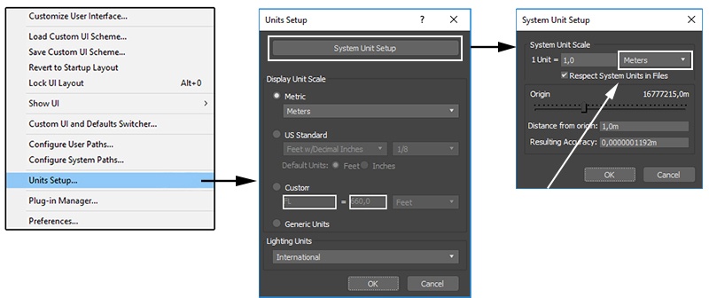
Go to Customize -> Units Setup and set Display Unit Scale to Metric Meters.
Also, set the System Units such that 1 Unit equals 1 Meter.
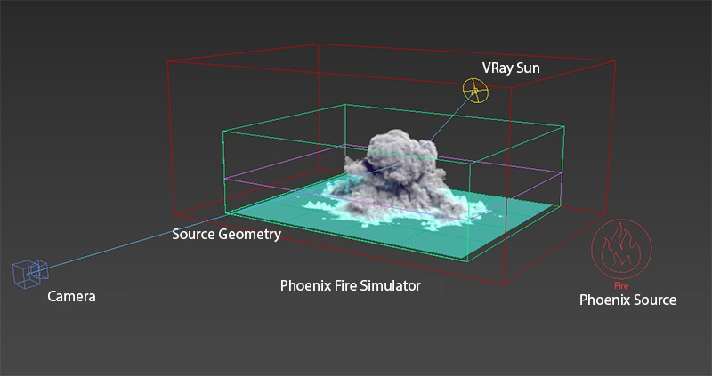
Scene Layout
The setup is fairly straight-forward.
The scene consists of a Polygon Plane with an applied Shell modifier (you should never use open geometry or geometry with no thickness as that could lead to all sorts of unpredictable issues). The Plane is textured with a Gradient Map and used as the emission geometry for the Phoenix FD Source. The Outgoing Velocity of the Source is animated to decrease over 24 frames.
Lighting is provided by the V-Ray Sun and the V-Ray Camera is used for the Exposure and Shutter Speed controls.
Phoenix FD Source Setup
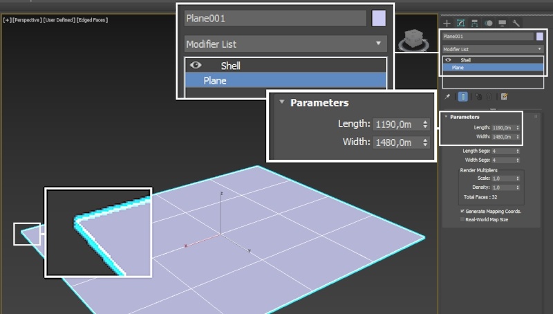
Create a plane from Standard Primitives → Plane and set its Length / Width parameters to 1190 / 1480 meters.
Apply a Shell modifier to the plane and set the Outer Amount to a low value. In this example, the Outer Amount is set to 2m.
The Shell modifier is applied to give the geometry thickness. This allows Phoenix FD to properly calculate the volume of the object that you're using for the emission.
We later limit the emission to only happen where the faces point in the +Z axis (in other words, the top of the shelled plane).
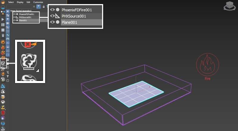
To save time, we start with the Large Scale Smoke preset on the Phoenix FD toolbar.
Select the shelled poly plane and Left-Mouse-Button click the Large Scale Smoke preset. This will automatically generate a Phoenix FD Source and Simulator, and will set up some Smoke rendering parameters for you. We will review those later when we're finished with the simulation.
Select the Phoenix FD Source and disable Temperature.
Animate the Outgoing Velocity such that it goes from [ 2000 at frame 0 ] to [ 0 at frame 20 ].
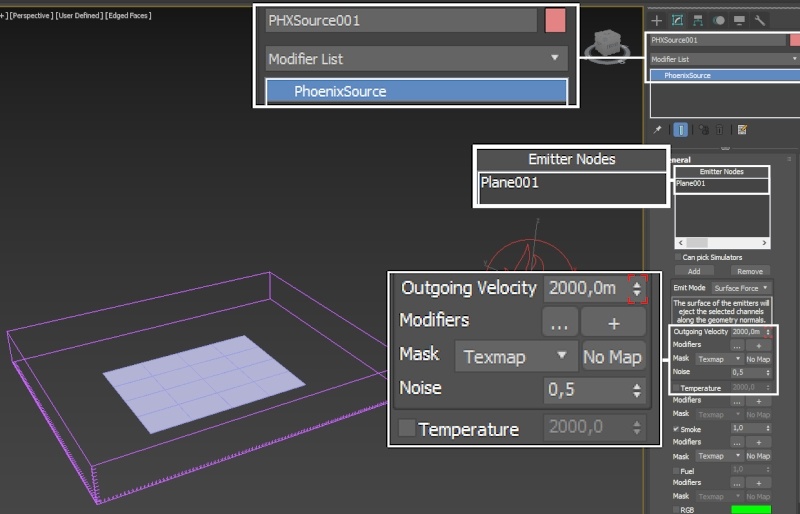
With the Phoenix FD Source still selected, click the map button to the right of the Mask parameter for Outgoing Velocity.
Select a Gradient Ramp as the mask. Set its Type to Radial - this produces a circular texture ideal for the base of the cloud.
Set the Noise parameters as shown in the screenshot. This will give you a randomized texture suitable for representing the shape of the cloud.
Changes to the Noise parameters will influence the cloud a lot so you may want to experiment with different settings once you've completed this tutorial.
Click the + icon under Outgoing Velocity to add a Discharge Modifier to the Phoenix FD Source. Discharge modifiers are a convenient way to control the strength of the emitter based on the position or orientation of your source object.
As mentioned earlier, only the top face of the shelled poly plane should be emitting smoke. Therefore, we set the Modify Outgoing Velocity by option to Normal Z, and the Space to World.
The ramp below is tweaked such that the left point is at [0.9, 0] and the right point is at [1, 1].
This means that only the faces which are nearly horizontal and pointing in positive Z will be used for emission. For more information on Discharge Modifiers, please check the Phoenix FD Discharge Modifiers documentation.
Right-Mouse-Button click the shelled poly plane and disable Solid Object from the Phoenix FD Properties.
Solid objects affect the calculation of velocity in the container by blocking the motion of fluids. In this case, the result would be better with the Solid option disabled.
Phoenix FD Simulator Setup
At the moment, the simulator box is far too large for our needs. In this setup, calculating the excess voxels is unnecessary and will only slow things down. Note that for some fire/smoke simulations it's good to keep a buffer of empty space around the simulated effect because the velocity simulation which drives the fire/smoke needs some additional space to unfold in a realistic way close to how nature works.
We also want the Simulator to expand up in the +Z direction to accommodate the shape of the cloud.
Select the Phoenix FD Simulator and open the Grid rollout.
Reduce the X / Y / Z size such that the Simulator tightly encompasses the shelled poly plane - as shown in the image.
Enable Maximum expansion and give the grid some extra voxels in all directions except for negative Z - we don't need the grid expanding down as that may ruin the shape of the cloud.
Reduce the Cell Size to ~4m. The Cell Size is the main "quality" control for the simulation - the lower this value is, the longer the simulation and the more detailed the result.
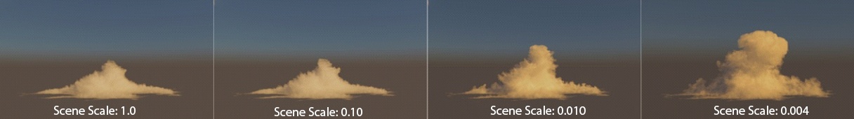
Set the Scene Scale to 0.004m. Because clouds are extremely large (a few kilometers in size) and moving very slowly, it would take prohibitively long to try to mimic the way the real world works. Instead, we reduce the time scale to a very short period of time (25 frames) and adjust the Scene Scale accordingly.
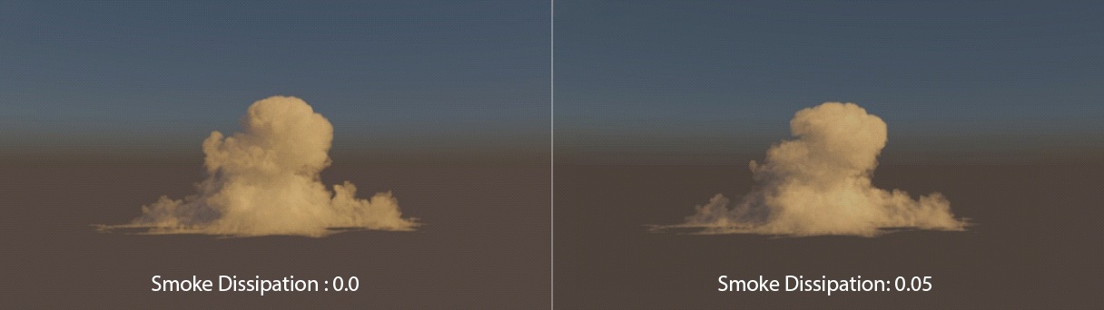
From the Dynamics rollout, set the Smoke Dissipation to 0.05. This will allow some of the smoke forming the cloud to slowly disappear, leaving behind interesting, swirly detail. The difference between a value of 0 and 0.05 is hard to notice so set this parameter as you see fit.
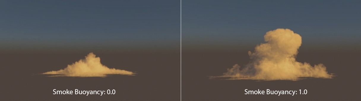
The Smoke Buoyancy should be set to 1. Buoyancy makes the fluid move upward, as if its pushed by a force from underneath. If you set this parameter to a negative value, the smoke will travel downward.
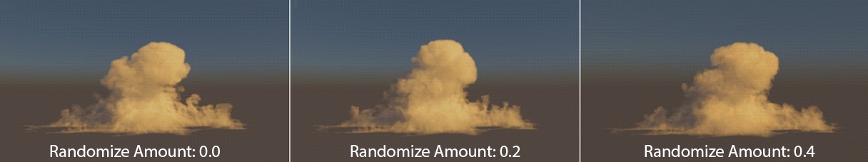
Set the Randomize Amount to 0.4 The Randomize options add random fluctuations in the fluid's velocity for each grid voxel. This should chip away at the cloud's volume, producing interesting perturbations.
Increase the Steps Per Frame to 7. Advection is the name of the process responsible for moving the Smoke along the calculated Velocity vectors on each frame. For fast-moving simulations, you need to raise the SPF so that you do not have a grainy appearance. As each simulated step removes details and also slows the simulation down, you shouldn't set the SPF higher than you need to and should increase it only if you see the smoke or fire become grainy when moving fast. On the flip side, the contents of the advected channel are more accurately transferred throughout the grid with higher SPF and the simulation moves more realistically.

We should now be ready with the simulation options. Press Start and let the simulation run for 20 or so frames.
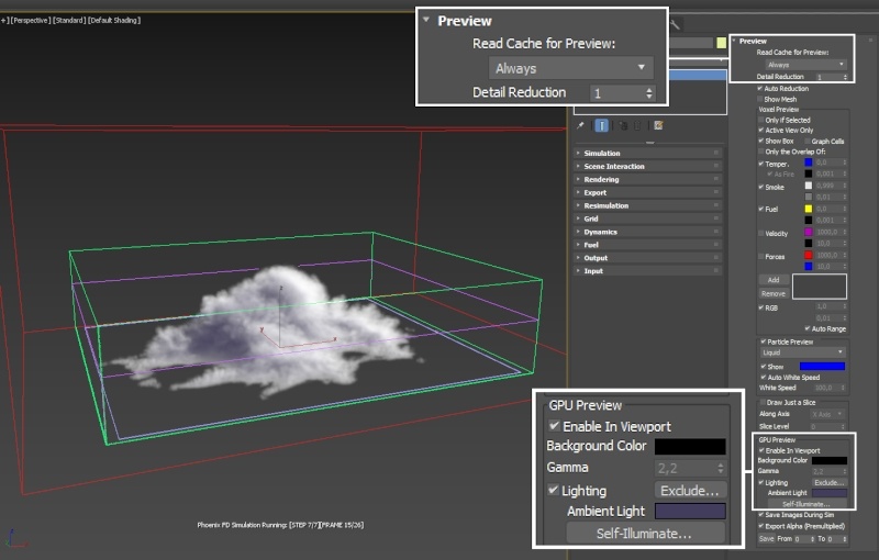
Phoenix FD provides a very high-quality viewport GPU Preview. Open the Preview rollout of the Simulator and select Enable In Viewport under the GPU Preview options.
Set the Ambient Light color to RGB [13, 11, 27] to get the cloud tinted in blue in the Viewport. Note that this setting has no effect on the Rendering.
Volumetric Rendering Settings
As you may have noticed, the cloud looks rather sparse. The Rendering options set up by the Large Scale Smoke preset we used as a starting point are tuned in a way that looks dense when the simulation quickly grows several times larger than the initial grid. However, since our cloud simulation mainly remains inside the initial grid, we need to change the render settings so that the smoke appears denser.
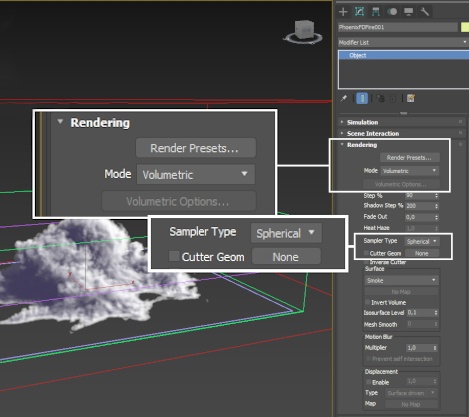
First of all, change the Sampler Type to Spherical. The Sampler Type parameter controls how individual voxels in the grid are interpolated. For instance, the Box type displays the cells as cubes and there is no blending between neighboring voxels. The Spherical type uses special weight-based sampling for the smoothest looking fluid and allows you to zoom in close to the grid without worrying about grid lines and voxels appearing in the render.
Head over to the Rendering rollout of the Simulator and click the Volumetric Options button. The window that pops up contains the majority of the volumetric shading parameters for Fire/Smoke simulations. You can think of it as a material/shader built into the Simulator.
Open the Smoke Opacity rollout and set the Based on parameter to Smoke. The cloud should now appear denser. Another way to do this would to be stay in Simple Smoke mode and to increase the Simple Smoke Opacity. The difference between the Smoke and Simple Smoke options is that the former provides you with an Opacity curve that you can edit. The Opacity Diagram is used to remap the Smoke channel - the X-axis is the input values from the simulation, and the Y-axis is the opacity output. It allows you to assign different opacity to the different densities of the Smoke. For instance, if you wanted to hide all the smoke that has a density of less than 0.5, you would move the left point of the graph to position [0.5, 0]. You can experiment by adding points on the graph and moving them around to see what effect they will have on the Viewport Preview. Simple Smoke mode is a simplified version of the Smoke mode where the Opacity Diagram is hidden and all you need to do is to adjust the Simple Smoke Opacity value which makes the smoke render thicker or thinner.
Open the Smoke Color rollout and make sure that the Based on parameter is set to Constant Color.
Set the Constant Color to pure white RGB : [255, 255, 255].
Set the Scattering mode to Ray-traced (GI only). Ray-traced scattering can only be rendered with Global Illumination enabled so make sure to turn it on from the V-Ray Render settings (should be On by default).
Ray-traced scattering tends to be slower than the Approximation methods which, as the name implies, try to speed up rendering by approximating with lower accuracy the appearance of light scattering in a volume. Ray-traced scattering, on the other hand, produces physically accurate scattering and the result tends to look better.
Lighting and Rendering
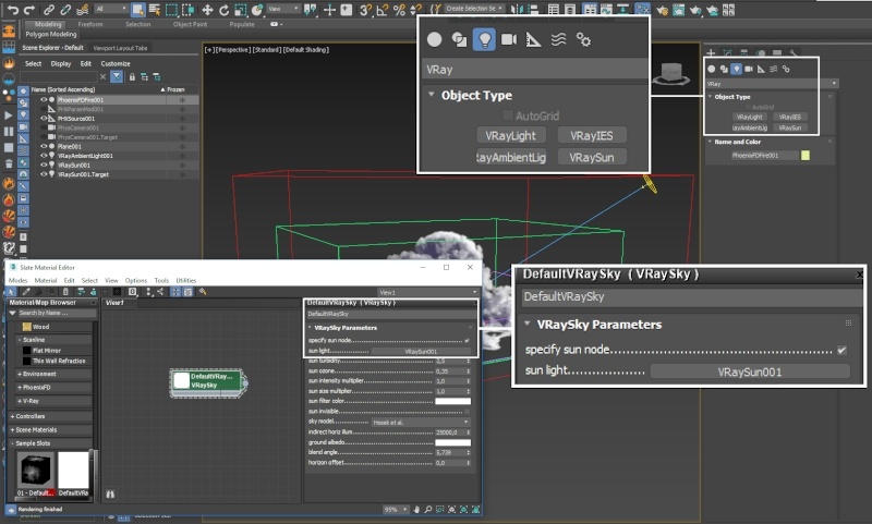
As this is an outdoor scene, a simple V-Ray Sun / Sky Setup should suffice.
The ground albedo parameter of the Sky Texture is set to white so the rendered ground looks better.
Optionally, you can link the Sun light to the Sky for physically accurate lighting by enabling the Specify sun node option on the V-Ray Sky texture. Then, create the link by simply Left-Mouse-Button clicking on the button next to the Sun Light parameter and selecting the V-Ray sun.
A standard Physical Camera is used for rendering.
The F-Number, Exposure and the Shutter Speed are the only changes made to the default settings.
F-Number is set to 8 and the Shutter Speed to Type: 1/seconds → 1/2000.
The light sensitivity under Exposure is set to Manual: ISO 100
Here are the Translation values for the camera and the sun, in case you'd like your scene to be 100% identical to the setup in the screenshots:
Sun Target: [ -31,19m, -63,68m, 133,82m ]
Sun: [ 841,315m , -719,656m, 852,844m ]
PhysCamera Target: [ 7,494m, 24,574m, 274,313m ]
PhysCamera: [ -314m, -2294,103m, 213,014m ]
VFB / Color Correction
You can use the V-Ray Frame Buffer to fine-tune the color of the rendered image.
We have provided a VFB corrections preset file for you called Cloud_VFB_corrections.vccglb. You can load it from the Frame Buffer Globals button → Load.
Using a LUT file is also a good option.
To the right is the rendered image with the provided color correction preset applied to the VFB.