This page provides a tutorial on creating a cloudscape with Phoenix for 3ds Max and Chaos Scatter.
Overview
This advanced tutorial guides you through the creation of daytime and night-time cloudscapes using Chaos Phoenix. It's recommended that you have at least basic knowledge in lighting, materials, and particle effects in 3ds Max.
This setup requires Phoenix 5.20.00, V-Ray 6 for 3ds Max 2019 and Chaos Scatter 2.5 or newer. You can download official Phoenix and V-Ray builds from https://download.chaos.com. If you notice a major difference between the results shown here and the behavior of your setup, please reach us using the Support Form.
This tutorial shows how to create a cloudscape that changes from a sunny day to a stormy night. We'll start by creating various cloud types, such as cumulus, anvil, and stratus. Then we will load them into multiple VRayVolumeGrids, integrated into a single scene. We will manually place a few hero clouds in the shot and then use Chaos Scatter to scatter some generic cloud assets over the region. Once we finish the cloudscape for the daytime scene, we will utilize PFlow to strike lightning from the clouds, for the stormy night scene.
For realistic cloud shading, we will tweak the value of the Phase Function of the simulators.
At the end of the tutorial, we will color-correct the image with the V-Ray Frame Buffer, and we will make the shots more cinematic by using V-Ray Light Mix. This allows us to adjust the key-to-fill light ratio without rendering the image again.
The final video is a mix of the daytime and night-time shots with a transition composite.
The Download button provides an archive of the scene files.
Workflow
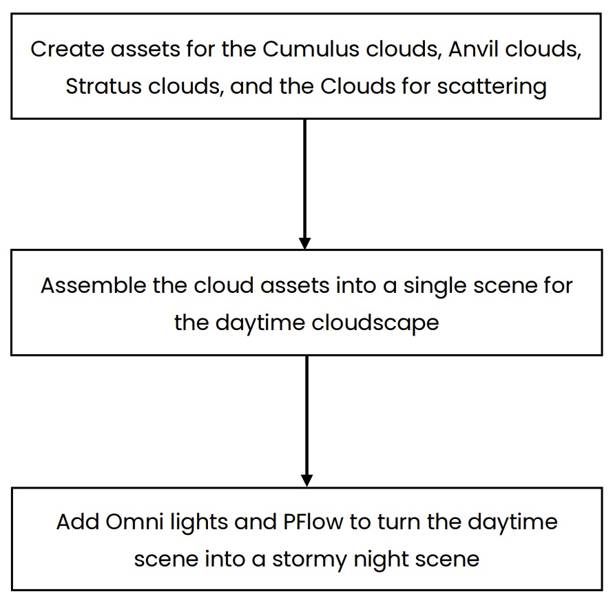
This is an extensive tutorial, which might be overwhelming at first glance. To make it easier to follow, we have created a workflow diagram that illustrates how the article is structured. The tutorial is divided into three major stages:
Asset creation: In this phase, we generate various cloud assets using Phoenix Fire/Smoke Simulators. This includes hero clouds such as Cumulus_A, Cumulus_B, and Anvil_Cloud. We also generate some generic clouds that will be scattered in the scene using Chaos Scatter in the next stage. These cloud assets are saved as *.aur cache files.
- Scene assembly: Once clouds of all types are ready, we load the *.aur files into one scene (cloudscape_daytime_start.max) using VrayVolumeGrid. First, we position our hero clouds and then fill the background and foreground with the generic clouds using Chaos Scatter. Finally, we create a VrayVolumeGrid for the environmental fog. We then render out the sequence for the daylight cloudscape.
- Lighting and particle effects: Next, we add some lighting effects using PFlow. We adjust the lighting conditions by adding some Omni lights and tweaking the Light Mix. We then render out the sequence as a stormy night.
To save time, you can download all the cloud assets from the Phoenix Cloud Assets page and start from the assembly part of this tutorial.
Units Setup
Scale is crucial for the behavior of any simulation. Large-scale simulations appear to move slower, while medium and small-scale simulations display lots of vigorous movement. When you create your Simulators, have a look at the Grid rollout where the real-world size of the Simulator is shown. If it cannot be changed, you can cheat the solver into working as if the scale is larger or smaller by changing the Scene Scale option in the Grid rollout.
The Phoenix solver is not affected by how you choose to view the Display Unit Scale - it is just a matter of convenience.
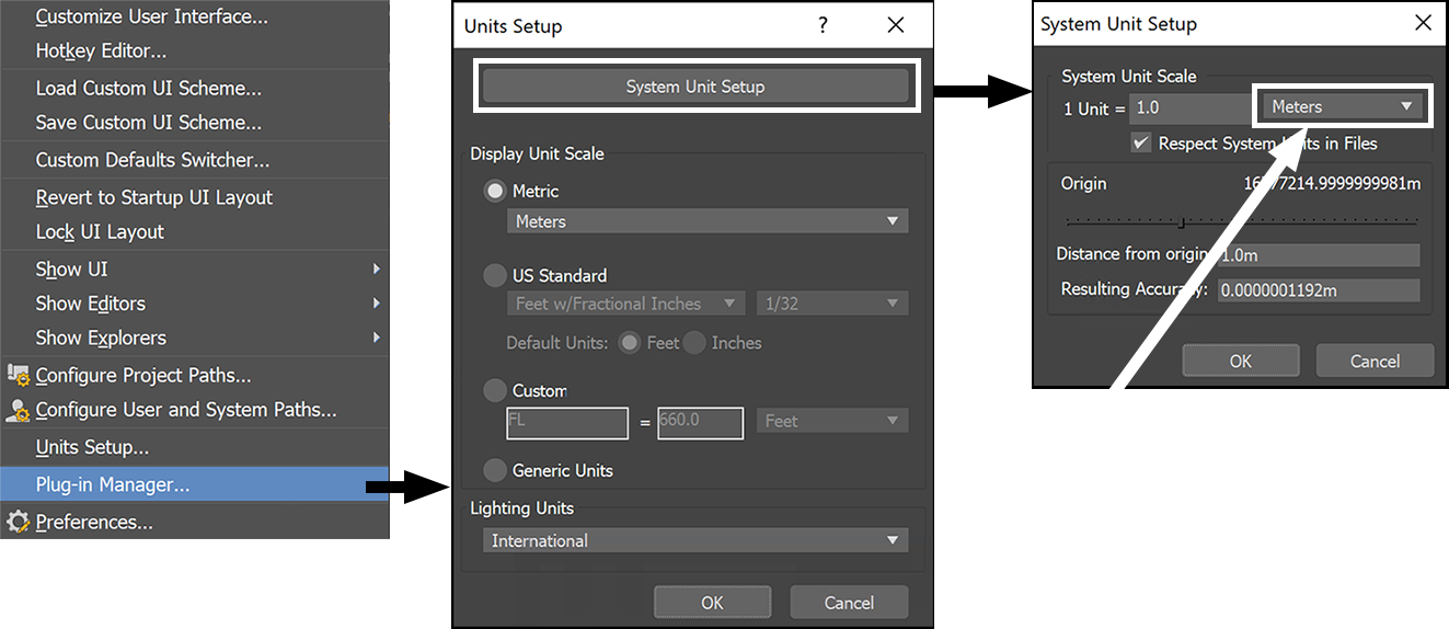
Since the height of a cumulus cloud is approximately 1000 meters, we have set the Scene Scale to Metric Meters.
- Go to Customize > Units Setup and set the Display Unit Scale to Metric Meters
- Set the System Units to 1 Unit = 1 Meter
Layout for the Final Assembly Scene
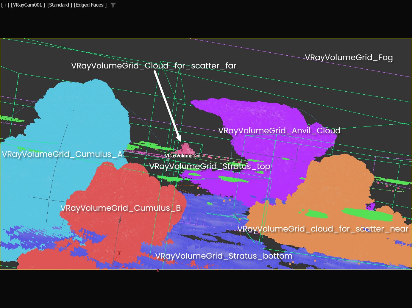
The final scene contains a total of seven VrayVolumeGrids, each loaded with an *.aur file for a specific type of cloud: Cumulus_A, Cumulus_B, Anvil_cloud, Cloud_for_scatter_near, and Cloud_for_scatter_far. Each VrayVolumeGrid has a different smoke color for easy identification. We have also added an extra VrayVolumeGrid for the environmental fog.
Note that we load the *.aur file into VrayVolumeGrid instead of a Phoenix Fire/Smoke Simulator. This way, the file can be used by V-Ray users who don't have Phoenix installed but still want to use the cloud assets in their project.
Although you can use the Phoenix Fire/Smoke Simulator to load the *.aur files, it is not recommended to mix V-Ray Volume Grid nodes and Phoenix Fire/Smoke Simulators in the same scene.
You should use only either Phoenix Simulators or V-Ray Volume Grids, otherwise the volumes might not blend properly.
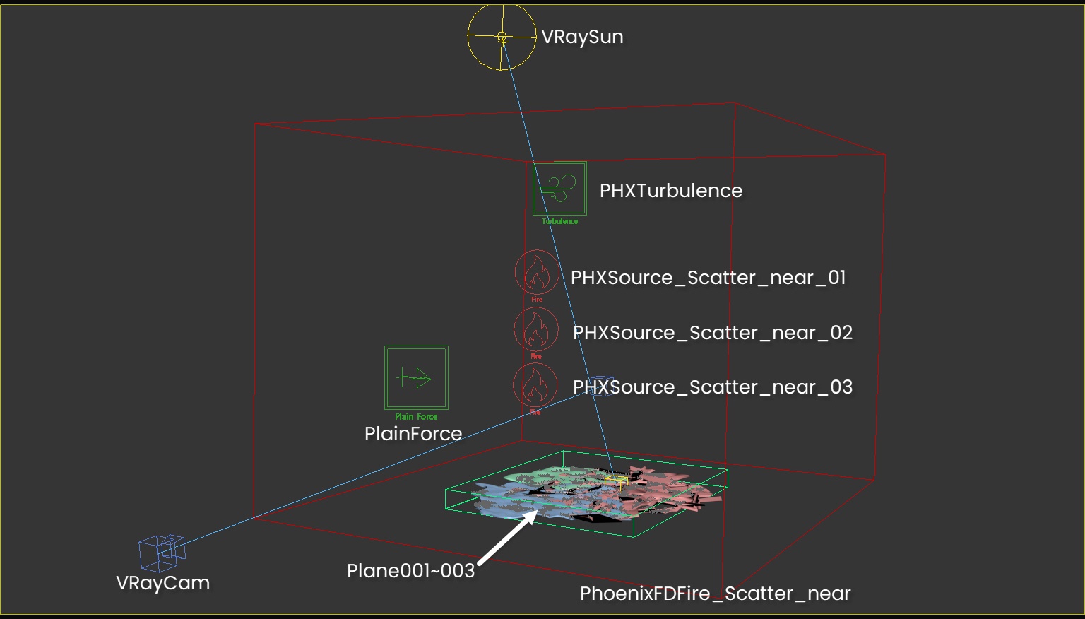
The final assembly scene contains the following elements:
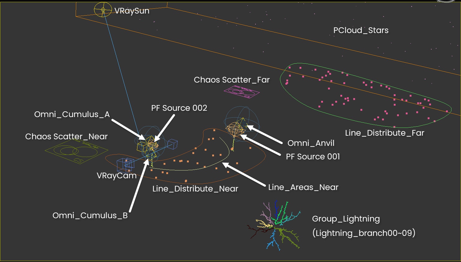
- VRayCam for rendering. The camera is tilted and animated as if we are on an airplane that is flying up.
- V-Ray Sun & Sky setup is used for the daytime scene lighting.
- Omni_Cumulus_A, Omni_Cumulus_B, and Omni_Anvil are for the stormy night scene. All of these Omni lights are animated to mimic a lightning effect.
- Two Chaos Scatter objects are used: one scatters the high-resolution Cloud_for_scatter_near in the foreground, and the other scatters the lower-resolution Cloud_for_scatter_far in the background.
- Line_Areas_Near and Line_Distribute_Near splines are used to define the region that Chaos Scatter_Near uses to scatter clouds. Line_Distribute_Far splines are used to define the region that Chaos Scatter_Far uses to scatter clouds.
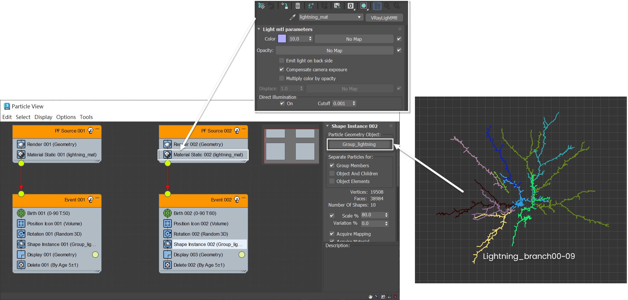
- Two Particle Flows are used for the night-time lightning: PF Source 001 is positioned within Anvil_cloud, while PF Source 002 is placed inside Cumulus_A. Both emit particles using Lightning_branch as shape instances.
- PCloud_Stars is used to create a background of stars.
For the day scene, we activate the Sun & Sky system and deactivate all the Omni lights.
For the night scene, we deactivate the Sun & Sky system and enable all the Omni lights. We also enable the PCloud in the background with two PFlow instances to produce lightning effects.
Additionally, as the lightning particles have a VRayLight material applied to them, they also have an illuminating effect.
Here are more details about the PFlow setup. As you can see, the particle system uses Group_Lightning as a Shape Instance. Both have VRayLightMtl applied, so their particles illuminate the scene.
Although these lighting meshes are static and do not have any growing animation, they are sufficient for the intended result.
Scene Setup
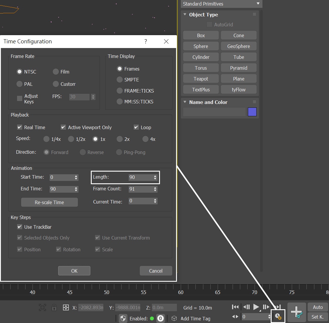
Click on the Time Configuration icon ( ![]() ) and set the Animation Length to 90, so that the Time Slider goes from 0 to 90.
) and set the Animation Length to 90, so that the Time Slider goes from 0 to 90.
This tutorial covers a range of steps for working with two different lighting scenarios. However, our focus here is on the specific steps related to working with Phoenix. You're welcome to use the camera and light settings provided in the sample scene.
If you would like to recreate these settings on your own, we've included the camera and light settings of the final renders below, for your reference.
Camera Settings
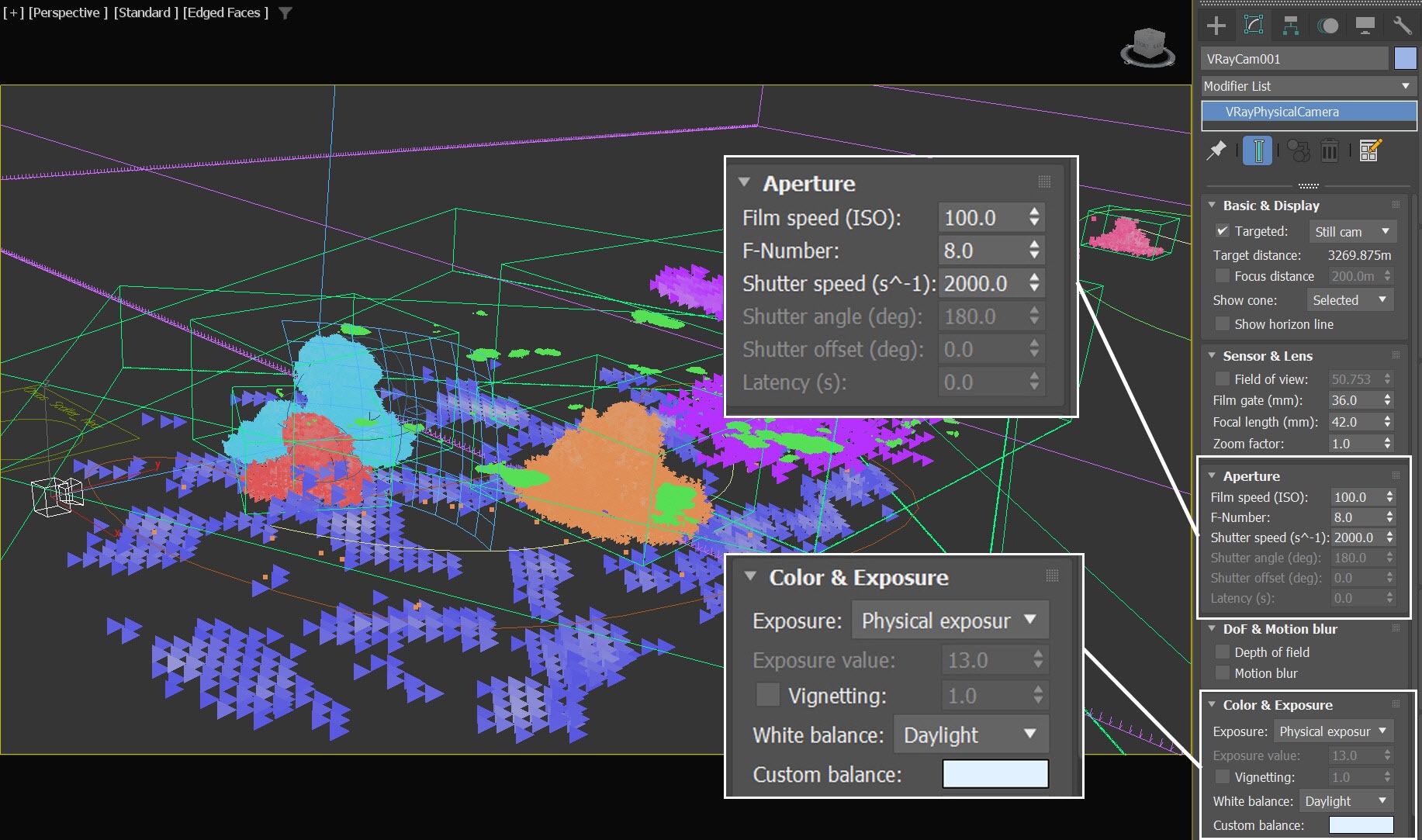
From Create Panel → Cameras → V-Ray, select the VRayPhysicalCamera and add it to the scene.
- The exact position of the Camera is XYZ:[1360.0, -3380.0, 768.0 ]
- The exact position of the Camera Target is XYZ:[ 1590.0, -120.0, 686.0 ]
- In the Aperture rollout:
Film speed is set to 100.0
F-Number is set to 8.0
Shutter Speed is set to 2000
- In the Color & Exposure rollout, White Balance is set to Daylight
Lighting for daytime
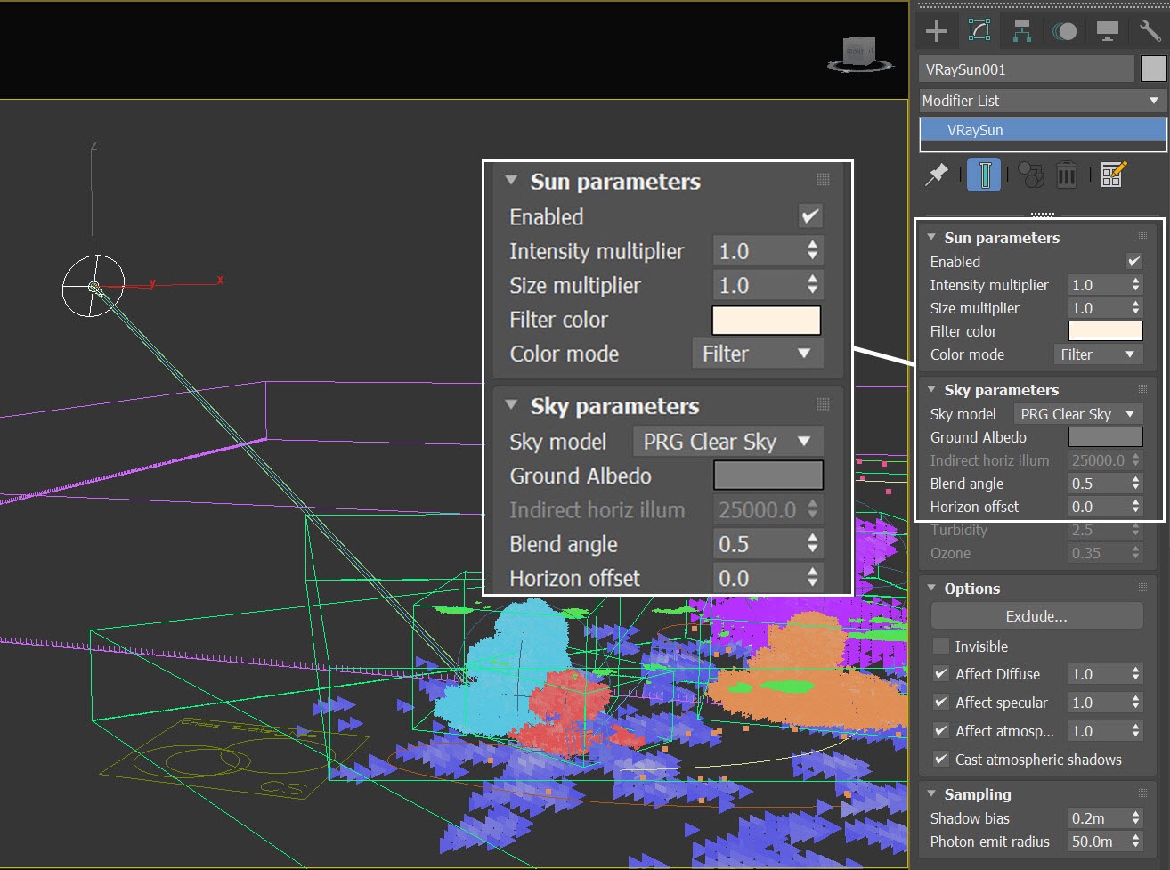
From the Create Panel go to Lights → V-Ray → VRaySun and create a VRaySun in the scene.
- The exact position of the VRaySun is set to XYZ:[ -7741.0, 6704.0, 4336.0]
- The exact position of the VRaySun Target is set to XYZ:[0.0, 0.0, 0.0 ]
- Set the Filter color to RGB(255, 227, 192)
Leave all other settings at their default values
The VRaySun's color was initially set to RGB(255, 255, 255), but it was later adjusted to RGB(255, 227, 192) using the To Scene feature with LightMix.
Lighting for stormy night
From the Create Panel, go to Lights → Standard → Omni and create three Omni lights in the scene. Rename them to Omini_Cumulus_A, Omini_Cumulus_B and Omni_Anvil, respectively.
Ensure accurate placement by positioning Omini_Cumulus_A inside Cumulus_A, Omini_Cumulus_B inside Cumulus_B, and Omni_Anvil inside Anvil_Cloud.
- For Omini_Cumulus_A, set its exact position to XYZ:[331.0, 175.0,308.0]. Adjust its Far Attenuation to Start at 304.0m and End at 749.0m. Control its Multiplier using a Noise Controller.
- For Omini_Cumulus_B, set its exact position to XYZ:[181.0, -578.0, 105.0]. Adjust its Far Attenuation to Start at 213.0m and End at 389.0m. Animate its Multiplier using keyframes.
- For Omni_Anvil, set its exact position to XYZ:[3002.0, 4488.0, 766.0]. Adjust its Far Attenuation to Start at 253.0m and End at 937.0m. Control its Multiplier using a Noise Controller.
- Set the color of all Omni lights to RGB(150, 191, 255).
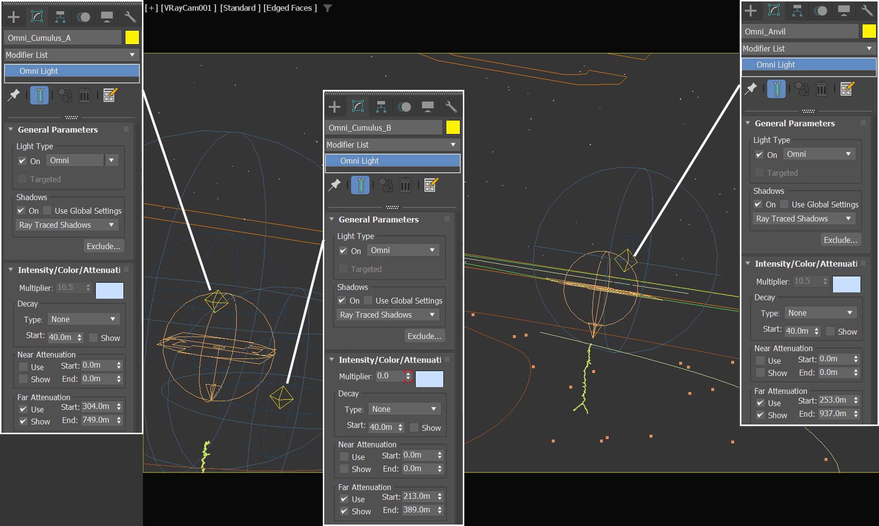
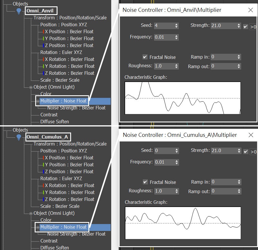
To mimic the blinking lightning, both Omni_Cumulus_A and Omni_Anvil have a Noise Controller applied to their Multiplier.
Adjust the following settings in the Noise Controller for Omni_Anvil:
- Set the Seed to 4
- Set the Strength to 21
- Set the Frequency to 0.01
- Enable the Fractal Noise option
Adjust the following settings in the Noise Controller for Omni_Cumulus_A:
- Set the Seed to 0
- Set the Strength to 21
- Set the Frequency to 0.01
- Enable the Fractal Noise option
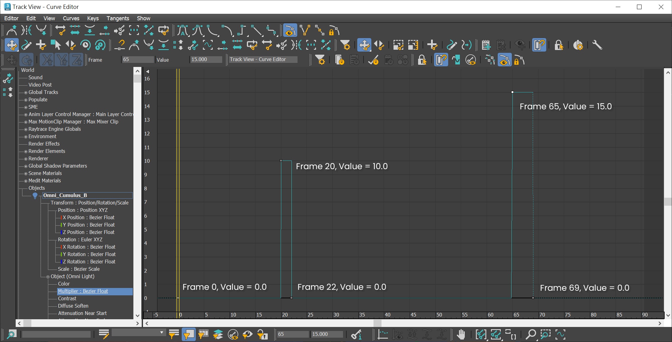
The Multiplier for Omni_Cumulus_B is animated manually using keyframes. Please refer to the screenshot for the specific frames and values.
Anatomy of the Cloudscape
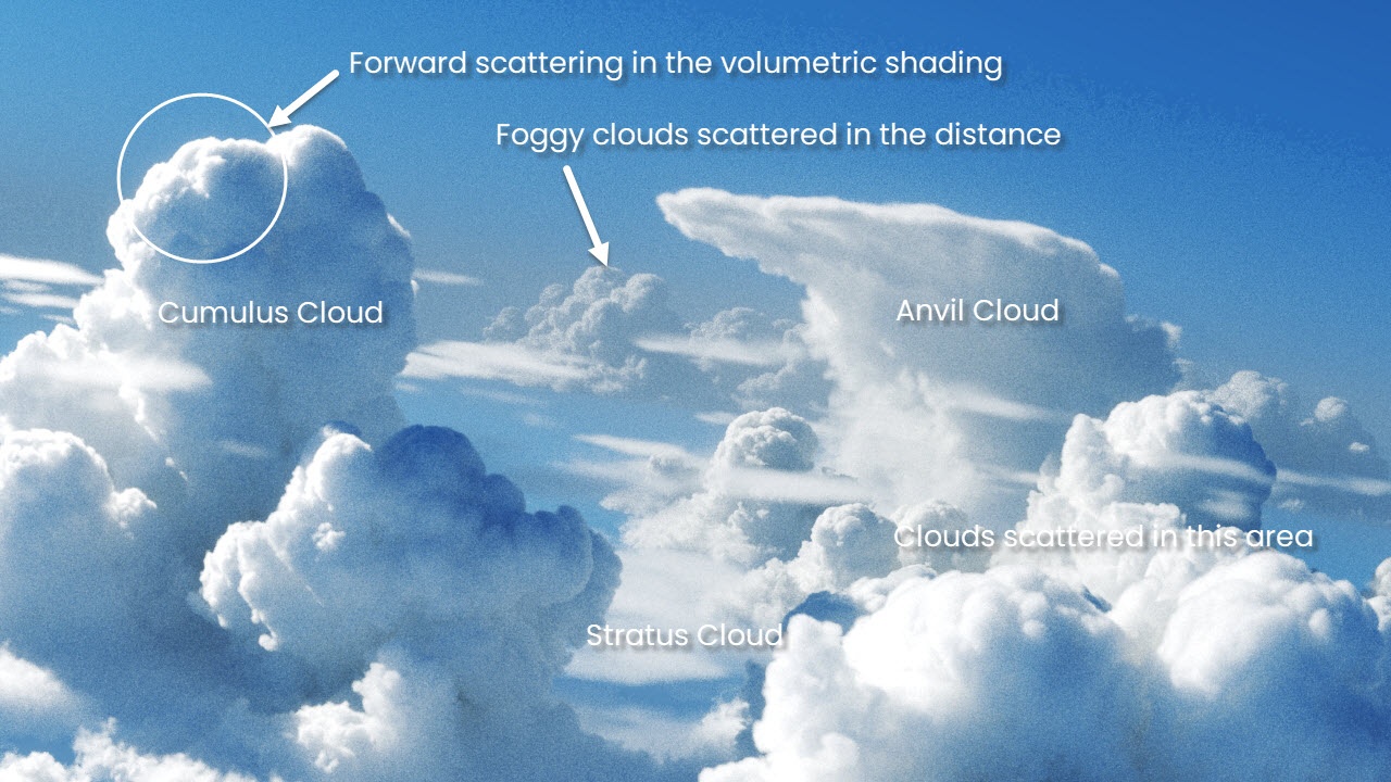
In the daytime scene, the middle ground is populated with highly-detailed cumulus and anvil clouds. Additionally, there are foggy clouds scattered in the distance, and some generic clouds scattered in the foreground. The stratus clouds intersect with these various types of clouds. The cloud shading is noteworthy, with beautiful and realistic forward scattering in its volumetric shading.
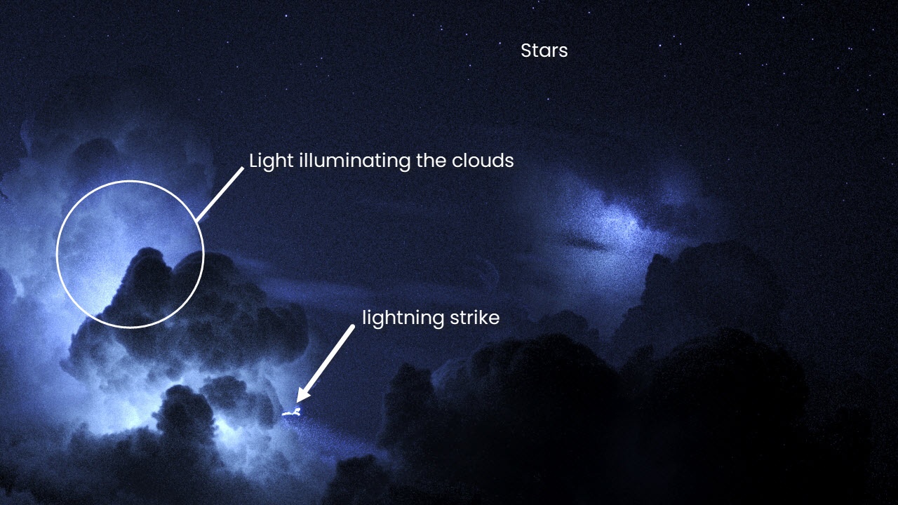
In the stormy night scene, the environment is foggier than during the daytime. Lights illuminate the large cumulus and anvil clouds. Lightning can be observed discharging from the clouds and flashing across the cloudscape.
Types of Clouds
Instead of scattering the same type of clouds throughout the sky, we are going to create three different types of clouds. This will enhance the realism of the cloudscape. We will create each of these assets in separate 3ds Max scenes and then assemble them in another dedicated scene.
The types of clouds we are going to create are cumulus, cumulonimbus (also known as anvil clouds), and stratus. Each of them looks different and is generated using a different method.
Cumulus | Anvil | Stratus | |
|---|---|---|---|
Morphology | Have flat bases and are often described as "puffy" in appearance | Cumulonimbus cloud that has reached stratospheric stability and has formed a characteristic flat, anvil-top shape. | Characterized by horizontal layering with a uniform base, as opposed to cumuliform clouds |
Emitted from | Plane with a Shell Modifier | Plane with a Shell Modifier | Sphere |
Source Emit mode | Surface Force | Surface Force | Volume Brush |
| Forces or other manipulation | Plain Force and PHXTurbulence | Plain Force, PHXTurbulence and Voxel Turner | |
| Examples | Cumulus_A, Cumulus_B, Cloud_for_scatter_near, and Cloud_for_scatter_far | Anvil_cloud | Stratus_top and Stratus_bottom |
Asset Creation
Creating the Cumulus_A cloud
Let's start creating assets for the scene, beginning with the main cumulus cloud - the Cumulus_A.
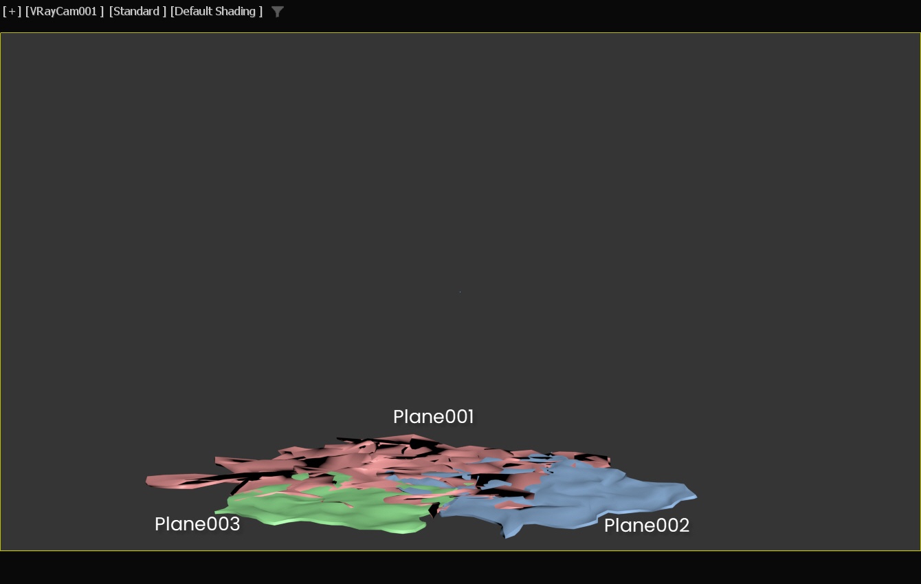
Please open the provided Cumulus_A_start.max scene file. To save you some time, we have prepared three planes in the scene, each with the Shell, Edit Poly, and Noise modifiers applied, needed to break up the emitted smoke and make the clouds more diverse and asymmetric.
We positioned these planes with some overlap between them. Each plane has a different size, to generate more interesting fluid results when we use them as emitter nodes. This allows the resulting cloud to look differently from all sides. If the cloud is scattered with Chaos Scatter, for instance, and if random rotation is assigned to each scattered cloud, you won't see obvious repetition or patterns.
In this section, we are going to create four cumulus cloud assets: Cumulus_A, Cumulus_B, Cloud_for_scatter_far, and Cloud_for_scatter_near. Since they are the same type of cloud and essentially share the same settings, to shorten the tutorial, we will only explain the procedure for making Cumulus_A. For the other cumulus clouds, we will skip through some of the steps and show the final setup.
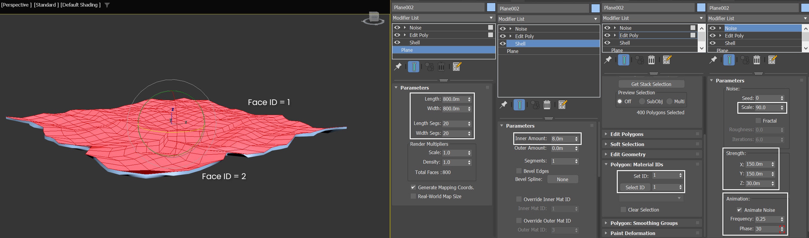
For example, we applied Shell, Edit Poly and Noise Modifiers to Plane002. While in Edit Poly mode, we select the top face of the geometry (marked in red), and set its face ID to 1. We set the face ID of the rest of the faces to 2.
The Phoenix Source in 3ds Max has the ability to use Polygon IDs as a 'mask' to selectively emit fluid only from faces with a given ID. In a later stage of the process, we will set the Polygon ID parameter to 1, ensuring that the Source emits solely from the polygons with an ID of 1.
This table shows the details of the three plane geometries with various modifier settings.
Feel free to tweak these settings to customize your cumulus cloud. You can adjust its size, position, or add stronger noise to the modifier. Changing these settings can lead to many opportunities for cloud variations after simulation.
Plane001 | Plane002 | Plane003 | |
|---|---|---|---|
Size | 1000X1000 | 800X800 | 600X600 |
Position | -125, 117, 0.0 | 300, -140, 0.0 | -290, -300, 0.0 |
Rotation | 0, 0, -30 | 0, 0, 30 | 0, 0, -20 |
Shell Modifier Inner Amount | 8.0 | 8.0 | 8.0 |
Noise Modifier Strength | 400, 400, 50 | 150, 150, 30 | 100, 100, 30 |
Noise Modifier Animate phase (The value of the phase is enclosed in parentheses.) | frame 0(0)~frame30(10) | frame 0(0)~frame30(30) | frame 0(0)~frame30(30) |
Fire/Smoke Simulation for Cumulus_A
Let's create a simulator now. Go to Create Panel > Create > Geometry > PhoenixFD > FireSmokeSim. Rename the simulator to PhoenixFDFire_Cumulus_A.
The exact position of the Phoenix Simulator in the scene is XYZ: [0.0, 0.0, -40.0].
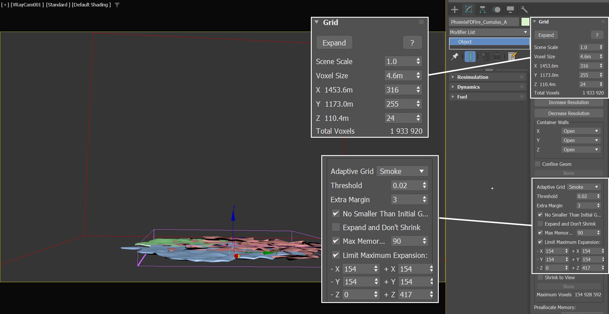
Open the Grid rollout and set the following values:
- Voxel Size: 4.6 m
- Size XYZ: [316.0, 225.0, 24.0]
- Expand the Container Walls, so that they match the sizes of the Grid's X, Y and Z parameters
- Set Adaptive Grid to Smoke. The Adaptive Grid algorithm allows the bounding box of the simulation to dynamically expand on-demand
- Set the Threshold to 0.02. This allows the simulator to expand when the Voxels near the walls of the simulation bounding box reach a Smoke value of 0.02 or greater
- Enable Limit Maximum Expansion and set its parameters accordingly:
X: (154, 154)
Y: (154, 154)
Z: (0, 417)
This saves memory and simulation time by limiting the Maximum Size of the simulation grid.
Renaming your simulator is essential, as the node name is also included in the names of the simulated cache files. With appropriate naming, you can easily organize different types of cloud assets in one location. This makes its easier to manage and access the assets in the future.
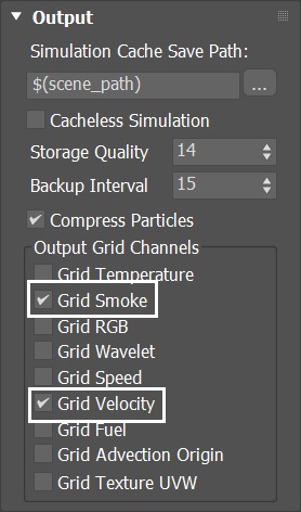
Output Settings
Select the Output rollout and enable the output of the Grid Smoke and Grid Velocity channels. We don't need the Temperature channel as we won't render fire.
Any channel used after the simulation is done, needs to be cached to disk. Such as:
- Velocity, which is required at render time for Motion Blur
- Wavelet, which is used for Wavelet Turbulence when performing a Resimulation
All the simulators in this tutorial utilize identical Output Settings. Keep in mind that this is the only time they will be mentioned in the tutorial, but the same settings need to be applied to all simulators in the scene.
Creating and Animating the Phoenix Fire/Smoke Sources in the Scene
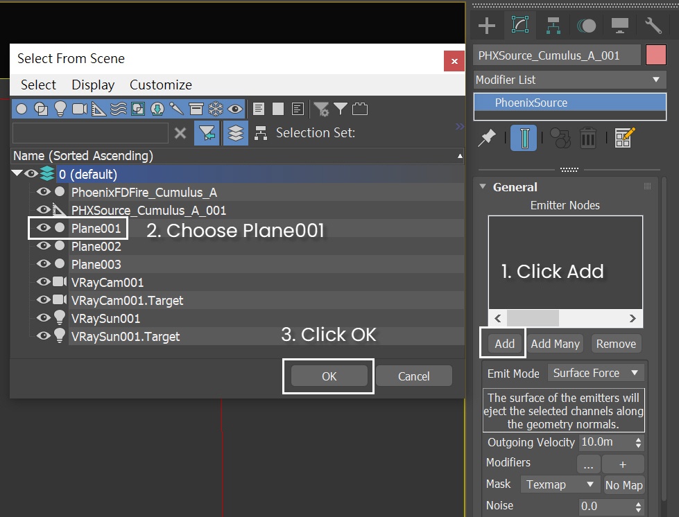
Go to Create Panel > Create > Helpers > PhoenixFD > PHXSource. Rename it to PHXSource_Cumulus_A_001.
Press the Add button and select the Plane001 geometry from the viewport or from the Scene Explorer.
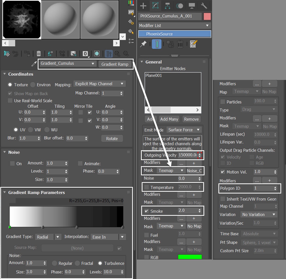
Set up the PHXSource_Cumulus_A_001's properties:
Set the Emit Mode to Surface Force
Disable the Temperature
Set the Smoke to 2.0
- Set the Outgoing Velocity's Mask type to Texmap
Set the Polygon ID to 1. This limits the emission only to faces with an ID of 1
Create a Gradient Ramp:
- Plug the map into the Outgoing Velocity's Texmap slot
- Rename it to Gradient_Cumulus
- Set the Gradient Type to Radial. This produces a circular texture ideal for the base of the cloud
- Set the Noise parameters:
Set the Noise Amount to 1.0
Set the Size to 5.0
Set the Noise type to Turbulence
- Add 2 extra flags to the gradient bar, so that there are a total of 4
- Set the Interpolation to Ease Out
- Edit the positions of the four flags on the gradient ramp using the table
Flag | Position | RGB | Interpolation |
|---|---|---|---|
1 | 0 | 255,255,255 | Ease In |
2 | 29 | 68,68,68 | Ease In |
3 | 60 | 5,5,5 | Ease In |
4 | 100 | 0,0,0 | Ease In |
Table of four flags on the gradient bar of the Gradient_Cumulus . Left (start point) to right (end point).
Changing the Noise parameters greatly influences the simulated cloud. It is recommended that you experiment with different settings once you've completed this tutorial. If you want to recreate the same result as shown here, follow the instructions exactly.
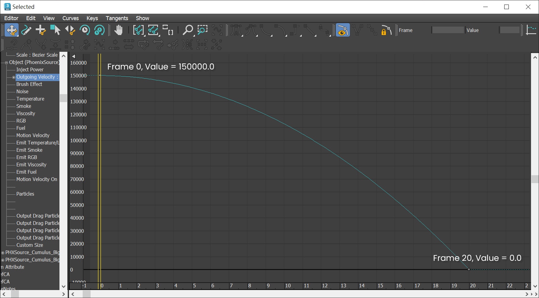
Animate the PHXSource_Cumulus_A_001's Outgoing Velocity
- Go to Graph Editors > Track View - Curve Editor
- Set keyframes for the Outgoing Velocity, so it can change over time. Each frame and value is shown in the screenshot and the table
Frame | Value | Tangent type |
|---|---|---|
0 | 150000.0 | Slow |
20 | 0.0 | Fast |
Keyframes for the FIre/Smoke Source's Outgoing Velocity
Set up Two More Sources for Cumulus_A
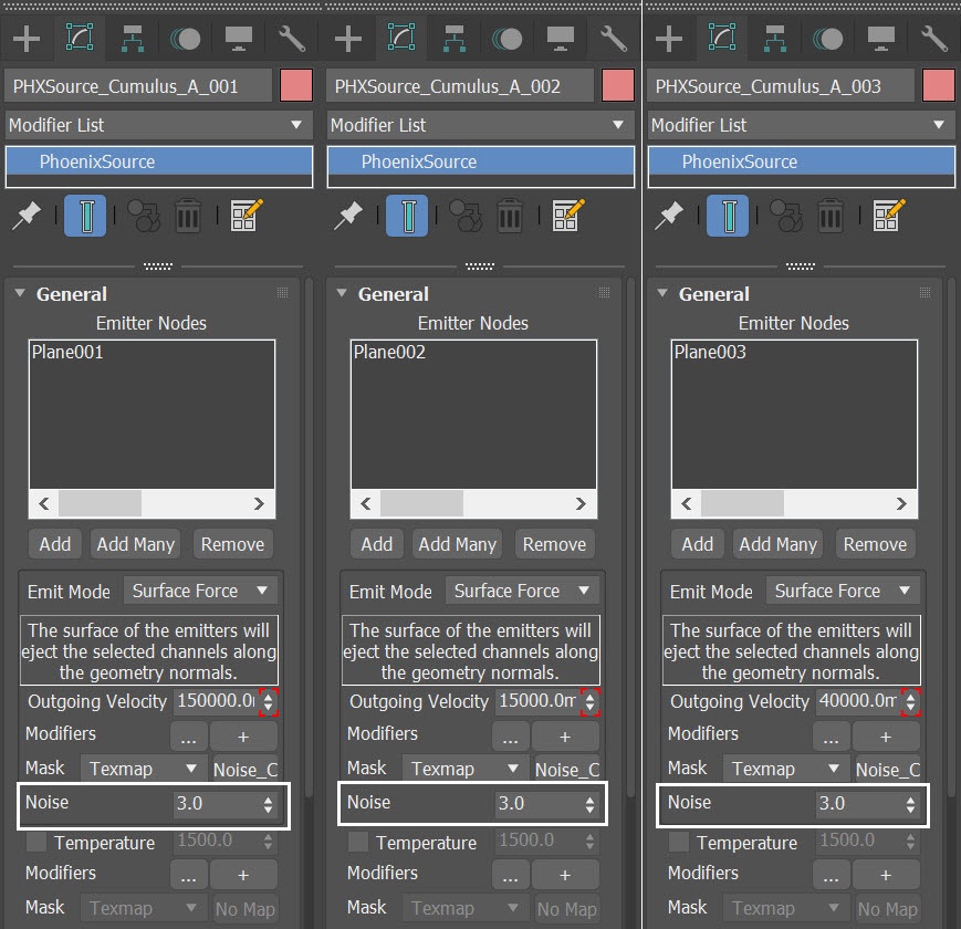
Repeat the same procedure for adding two more Phoenix Sources in the scene. Rename them to PHXSource_Cumulus_A_002 and PHXSource_Cumulus_A_003, respectively. Add Plane002 to the emitter nodes in PHXSource_Cumulus_A_002 and add Plane003 to PHXSource_Cumulus_A_003's emitter nodes.
Use the table to adjust the Outgoing Velocity of the Phoenix Sources.
PHXSource_Cumulus_A_01 | PHXSource_Cumulus_A_02 | PHXSource_Cumulus_A_03 | |
|---|---|---|---|
Emitter Nodes | Plane001 | Plane002 | Plane003 |
Outgoing Velocity at Frame 0 (Tangent type to Slow) | 150000.0 | 15000.0 | 40000.0 |
Outgoing Velocity at Frame 20 (Tangent type to Fast) | 0.0 | 0.0 | 0.0 |
Initial Simulation for the Cumulus_A
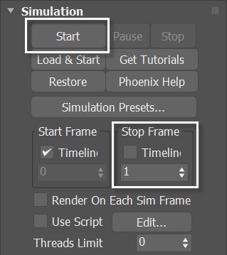
Select the Simulation rollout of the PhoenixFDFire_Cumulus_A Simulator. We only need to simulate 10 frames, so set the Stop Frame to 10. Press the Start button to simulate.

This is a voxel preview of the current animation. The cloud appears too short.
Increase Steps Per Frame
In the Dynamics rollout of the simulator, increase the Steps Per Frame to 10. Run the simulation again. The Source emits fluid with very high velocity, so more Steps Per Frame are needed to capture it better.
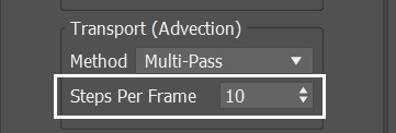
This is the voxel preview of the current animation. As you can see, the height of the cloud has increased significantly.
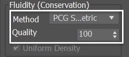
Switch to the PCG Solver
Select the PhoenixFDFire_Cumulus_A Simulator and in the Dynamics rollout change the Fluidity Method to PCG Symmetric, with a Quality of 100. Run the simulation again.
The PCG Symmetric option is the best method for smoke or explosions in general, preserving both detail and symmetry. The high Conservation Quality allows the smoke to swirl better. For more information, visit the Conservation documentation.
This voxel preview shows the current animation.
Delete Faces of Plane001
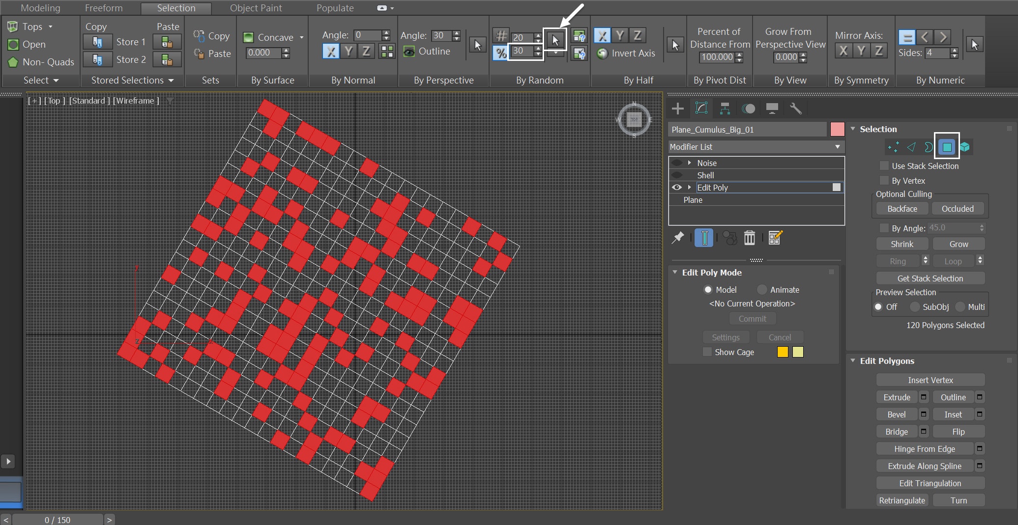
To define the shape of the cloud more, let's edit the model of Plane001. First, select Plane001 and go to the Modifier panel. Then, add an Edit Poly Modifier and navigate to the Selection rollout. Click on the Polygon button, and then use the Ribbon's By Random option to randomly delete 30% of the faces.
After deleting, assign a Polygon ID of 1 to the top faces, and set an ID of 2 for the rest of the faces. Finally, run the simulation again to see the updated cloud shape.
In this case, deleting some faces of Plane001 creates a more defined shape and enhances the visibility of the puffs in the cloud morphology, as it prevents them from clumping together.
Deleting some faces also allows for cloud variations. By deleting different faces, you can achieve different appearances of the clouds.
This voxel preview shows the current animation. Now we see a more defined shape of a cumulus cloud.
Introduce Noise
To create a more natural-looking cloud, we can add some noise to the simulation. To achieve this, let's increase the Noise value for the Outgoing Velocity to 3.0 for all three PHXSources in the scene.
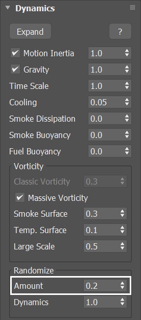
Additionally, select PhoenixFDFire_Cumulus_A and navigate to the Dynamics rollout to increase the Randomize Amount to 0.2.
Run the simulation again.
This voxel preview shows the current animation. Now we have a more organic-looking cloud.
Adding Phoenix Turbulence
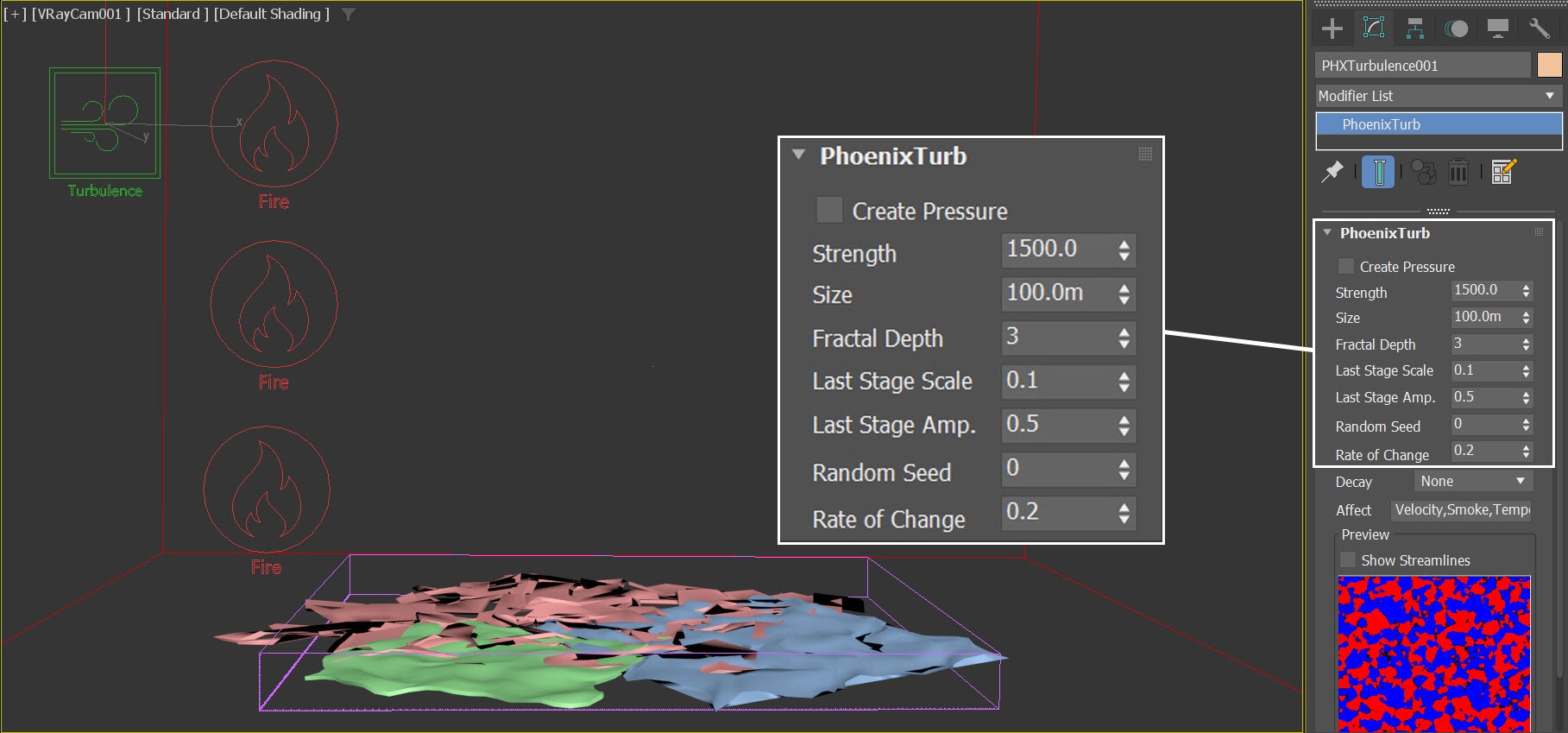
To bring more realism to the cloud, let's add some forces to the scene. Go to the Create panel > Helpers > PhoenixFD and click on PHXTurbulence. Create a Phoenix Turbulence in the scene.
- Set the position to XYZ: [-850.0, -872.0, 1200.0]
- Set the Strength to 1500.0
- Set the Size to 100.0m. Keep in mind that the Simulator's width exceeds 1000m in both X and Y directions, so this would create curls that are about 10% of the simulator size.
- Set the Fractal Depth to 3.0
- Reduce the Rate of Change to 0.2
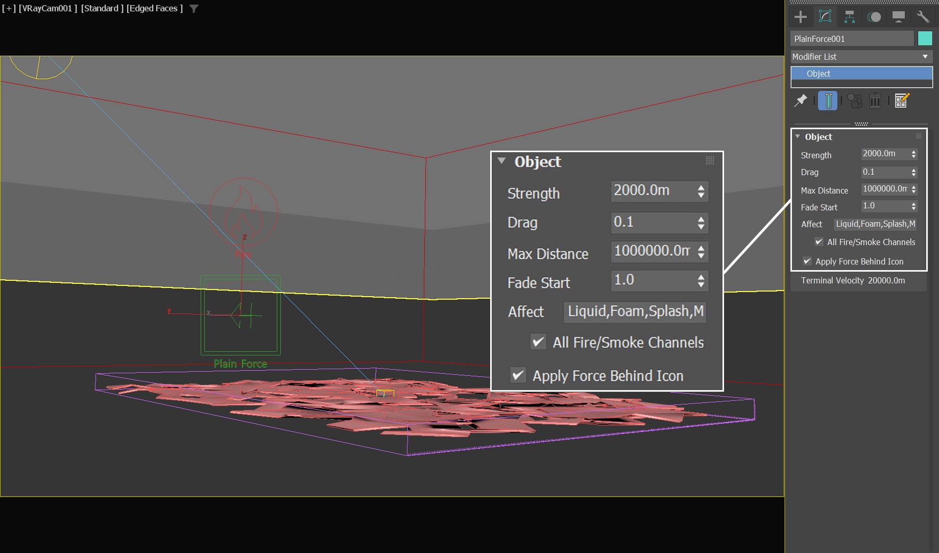
Adding Plain Force
Then we add a Phoenix Plain Force, a simple directional force in the scene. Go to Create panel > Helpers > PhoenixFD and add a Phoenix Plain Force in the scene.
Set the following parameters:
The exact position of the Plain Force in the scene is XYZ: [126.0, -1500.0, 560.0]
Rotate the Plain Force to XYZ: [-90.0, 0.0, 0.0]. Set its Strength to 200.0m
Set the Drag to 0.1
Enable the Apply Force Behind Icon option
Final Simulation of the Cumulus_A
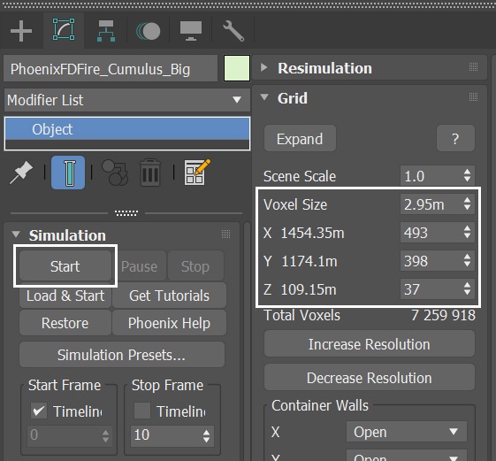
Now we are ready for the final simulation. Let's increase the grid resolution of the simulator. Make the following changes:
- Voxel Size: 2.95 m
- Size XYZ: [493, 398, 37 ]
With the new grid resolution and forces in the scene, click on Start to run the final simulation for Cumulus_A.
This voxel preview shows the final animation.
Run a test render of frame 10 with the default volumetric settings. This helps assess what changes are needed to improve the look of the simulation.
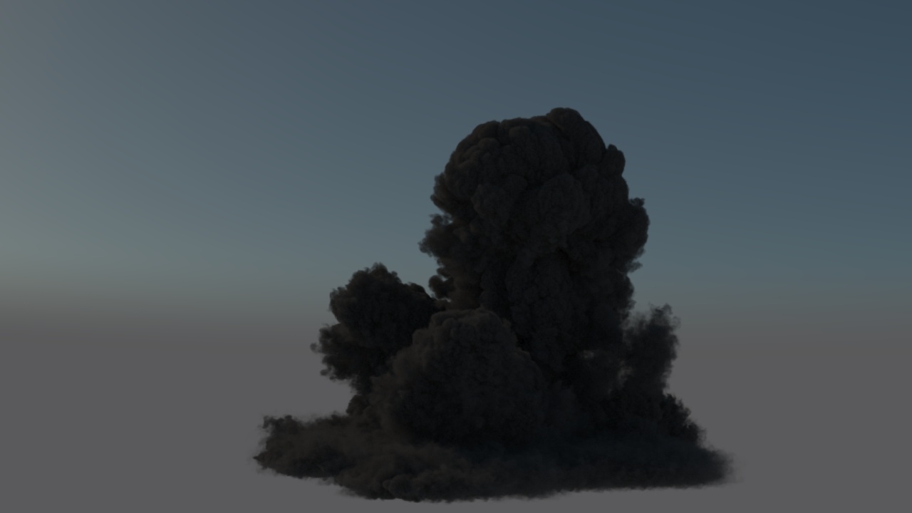
Improve the Volumetric Settings
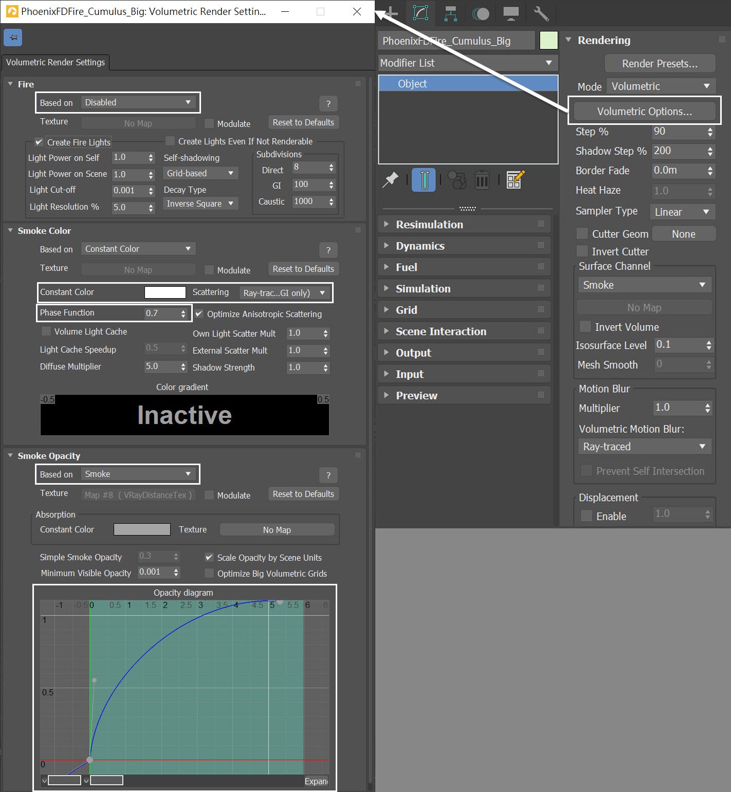
Select the PhoenixFDFire_Cumulus_A Simulator and go to its Volumetric Render Settings.
- Set the Fire Based on option to Disabled - we won't need any fire in this scene.
- Change the Smoke Color to pure white of RGB (255, 255, 255). This allows for the strongest light scattering inside the cloud.
- Set the Scattering to Ray-tracing (GI only) - this mode uses physically accurate scattering of light rays and produces the most realistic results. However, It is slower to render.
- Set the Smoke Opacity's Based on option to Smoke.
- Adjust the curve for the smoke to match the screenshot.
Increasing the value for Light Cache Speedup speeds up the render, but it also lowers the quality of the Volume Light Cache. If dark cubic grid artifacts start forming on the smoke, the parameter is set too high. For more information, visit the Volumetric Rendering In-Depth page.
In this case set the Volume Light Cache to disabled as it will produce cleaner render result.
In the Rendering rollout, set the Sampler Type to Spherical. The Sampler Type determines the blending method between adjacent grid voxels and is used to balance between render speed and quality. In this case the Spherical sampler gives us the highest-quality result.
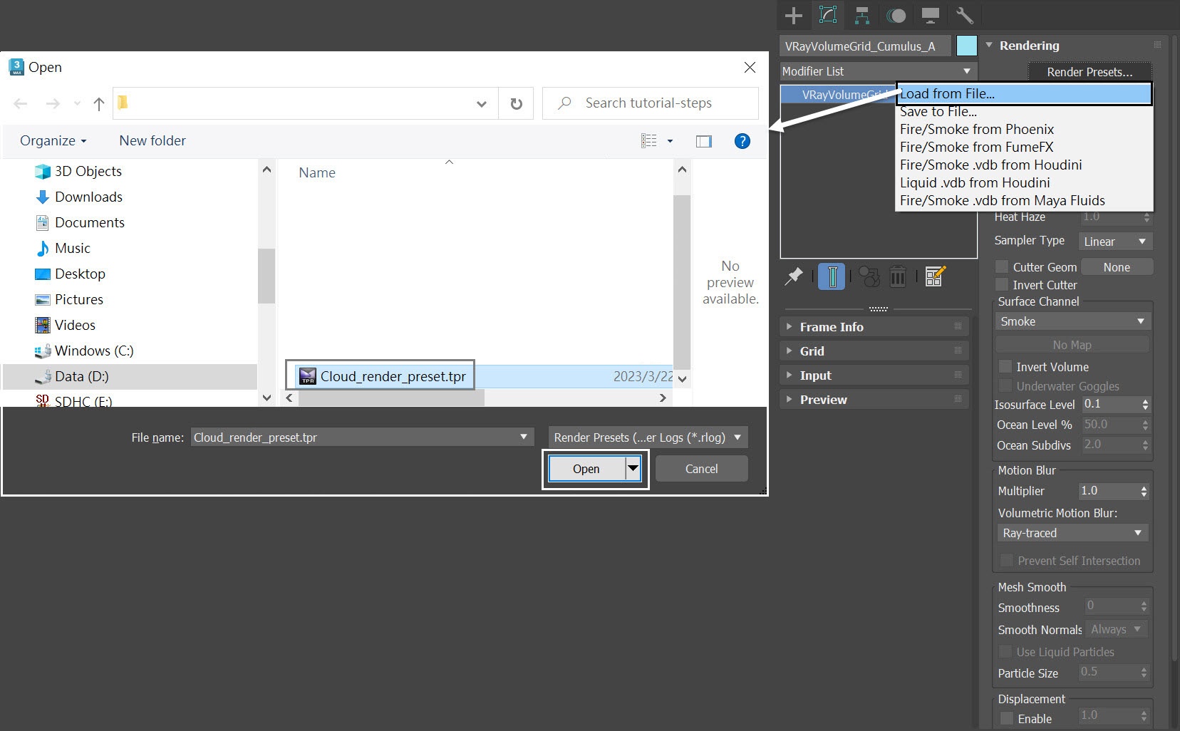
Alternatively, you can load up a render preset from the Cloud_render_preset.tpr file, that is provided in the sample scene.
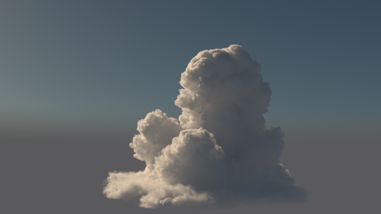
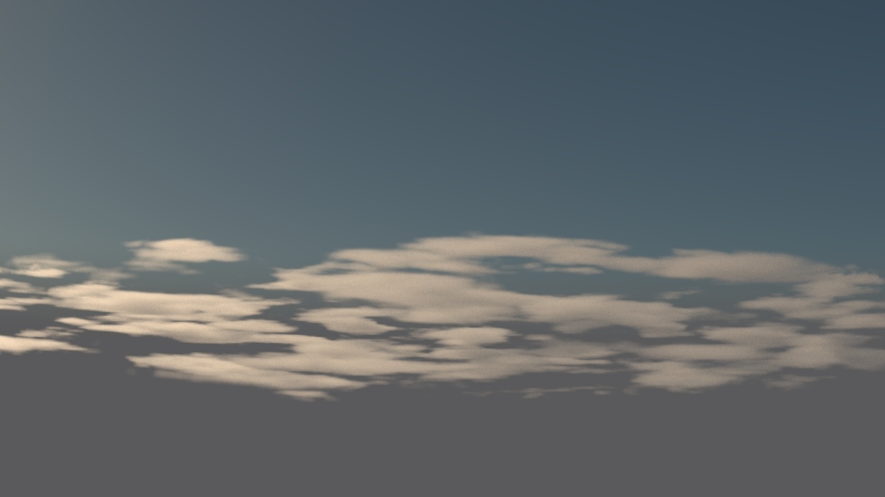
With the new volumetric settings , run a test render of frame 10. This is the asset for Cumulus_A.
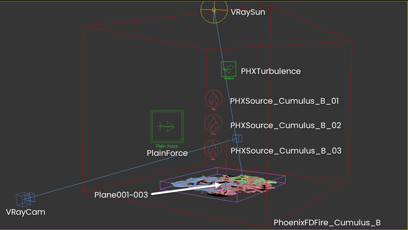
Creating the Cumulus_B Cloud
There's already one cumulus cloud in the scene. Now we will create another variant for the same type. You can open the scene "Cumulus_B_final.max" and save time, as we have already prepared all the required elements and configured the settings there. It is essentially similar to Cumulus_A.
This table shows the details for all three plane geometries in the scene.
Similar to the setup in Cumulus_A, Plane001 here also has 30% of its faces removed.
Plane001 | Plane002 | Plane003 | |
|---|---|---|---|
Size | 1000X1000 | 800X800 | 600X600 |
Position | 249, -14, 0.0 | 485, -296, 0.0 | -56, 28.0, 0.0 |
Rotation | 0, 0, -30 | 0, 0, -5 | 0, 0, -20 |
Shell Modifier Inner Amount | 8.0 | 8.0 | 8.0 |
Noise Modifier Strength | 400, 400, 50 | 150, 150, 30 | 100, 100, 30 |
Noise Modifier Animate phase (The value of the phase is enclosed in parentheses.) | frame0 (0)~frame30(10) | frame0 (0)~frame30(30) | frame0 (0)~frame30(30) |
This table shows all the settings for the three PHXSouces in the scene.
The gradient map that we utilized to mask the Outgoing Velocity is identical to the one used in Cumulus_A.
PHXSource_Cumulus_B_01 | PHXSource_Cumulus_B_02 | PHXSource_Cumulus_B_03 | |
|---|---|---|---|
Emitter Nodes | Plane001 | Plane002 | Plane003 |
| Mask for Outgoing Velocity | Gradient_Cumulus | Gradient_Cumulus | Gradient_Cumulus |
| Noise for Outgoing Velocity | 3.0 | 3.0 | 3.0 |
Outgoing Velocity at Frame 0 | 150000.0 | 15000.0 | 40000.0 |
Outgoing Velocity at Frame 20 | 0.0 | 0.0 | 0.0 |
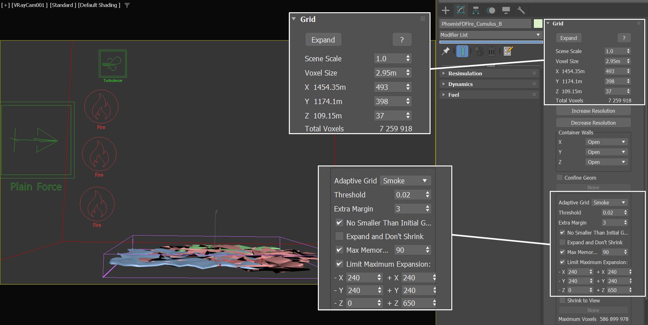
Here are the settings for the simulator - PhoenixFDFire_Cumulus_B:
The exact position of the Phoenix Simulator in the scene is XYZ: [308.0, -116.5 -40.0].
Open the Grid rollout and set the following values:
- Voxel Size: 2.95 m
- Size XYZ: [493, 398, 37]
- Expand the Container Walls, so that they match the sizes of the Grid's X, Y and Z parameters
- Set the Adaptive Grid to Smoke. The Adaptive Grid algorithm allows the bounding box of the simulation to dynamically expand on-demand
- Set the Threshold to 0.02. This allows the simulator to expand when the Voxels near the corners of the simulation bounding box reach a Smoke value of 0.02 or greater
- Enable Limit Maximum Expansion and set its parameters accordingly:
X: (240, 240)
Y: (240, 240)
Z: (0, 650)
This saves memory and simulation time by limiting the maximum size of the simulation grid.
The simulator is loaded along with the Cloud_render_preset.tpr, so the volumetric settings are all set for the final render.
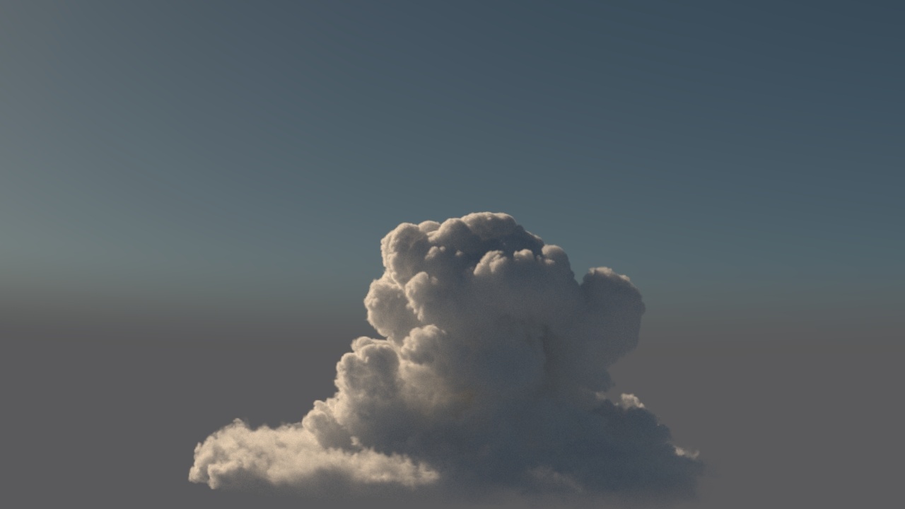
Select the Simulation rollout of the PhoenixFDFire_Cumulus_B Simulator. We only need to simulate 7 frames, so set the Stop Frame to 7. Press the Start button to simulate.
Run a test render of frame 7. This is our asset for the Cumulus_B cloud.
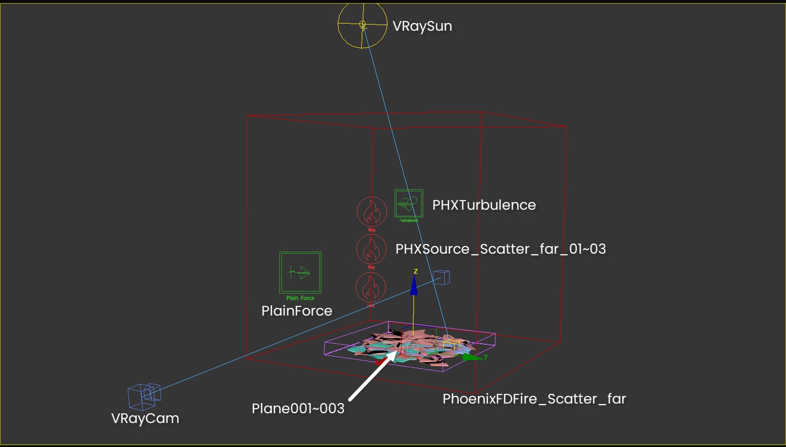
Creating the Scatter_far Cloud
Open the scene "Cloud_for_scatter_far_final.max", where we have already prepared all the necessary elements and configured the settings for you. The setup is essentially the same as the previous two. However, the main difference is that since it is far from the camera, this cloud has a low-resolution grid to optimize performance.
This table shows the details for all three plane geometries in the Cloud_for_scatter_far scene.
Plane001 | Plane002 | Plane003 | |
|---|---|---|---|
Size | 885 X 975 | 500 X 529 | 615 X 615 |
Position | 62, -318, 0.0 | 36, -93, 0.0 | 339, -358, 0.0 |
Rotation | 0, 0, 0 | 0, 0, 30 | 0, 0, -20 |
Shell Modifier Inner Amount | 8.0 | 8.0 | 8.0 |
Noise Modifier Strength | 400, 400, 50 | 150, 150, 30 | 100, 100, 30 |
Noise Modifier Animate phase (The value of the phase is enclosed in parentheses.) | frame0 (0)~frame30(10) | frame0 (0)~frame30(30) | frame0 (0)~frame30(30) |
This table shows all the settings for the three PHXSouces in the scene.
The gradient map that we utilize to mask the Outgoing Velocity is identical to the one used in Cumulus_A.
PHXSource_Scatter_far_01 | PHXSource_Scatter_far_02 | PHXSource_Scatter_far_03 | |
|---|---|---|---|
Emitter Nodes | Plane001 | Plane002 | Plane003 |
| Mask for Outgoing Velocity | Gradient_Cumulus | Gradient_Cumulus | Gradient_Cumulus |
| Noise for Outgoing Velocity | 3.0 | 3.0 | 3.0 |
Outgoing Velocity at Frame 0 | 150000.0 | 15000.0 | 40000.0 |
Outgoing Velocity at Frame 20 | 0.0 | 0.0 | 0.0 |
Here are the settings for the PhoenixFDFire_Scatter_far Simulator:
The exact position of the Phoenix Simulator in the scene is XYZ: [95.0, -327.0 -40.0]
Open the Grid rollout and set the following values:
- Voxel Size: 5.8 m
- Size XYZ: [197, 190, 19]
- Expand the Container Walls, so that they match the sizes of the Grid's X, Y and Z parameters
- Set Adaptive Grid to Smoke. The Adaptive Grid algorithm allows the bounding box of the simulation to dynamically expand on-demand
- Set the Threshold to 0.02. This allows the simulator to expand when the Voxels near the corners of the simulation bounding box reach a Smoke value of 0.02 or greater
- Enable Limit Maximum Expansion and set its parameters accordingly:
X: (80, 80)
Y: (80, 80)
Z: (0, 325)
This saves memory and simulation time by limiting the maximum size of the simulation grid.
The simulator is loaded along with the Cloud_render_preset.tpr, so the volumetric is all set for the final render.
To optimize performance, we used a very low resolution for the simulator, since the cloud is placed far away from the camera.
To increase flexibility, an alternative approach is to simulate the cloud with a higher grid resolution and then use the Cache Converter tool and decrease the grid resolution of the cache files. This enables the simulated caches to be used for both close-up and far-away clouds, allowing for on-demand optimization of render performance through the tool.
Select the Simulation rollout of the PhoenixFDFire_Scatter_far Simulator. We only need to simulate 4 frames, so set the Stop Frame to 4. Press the Start button to simulate.
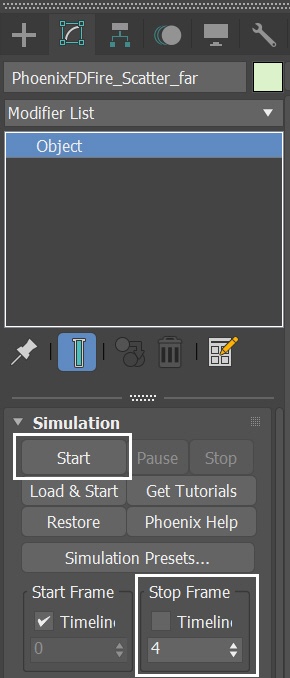
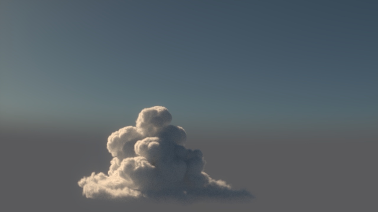
Run a test render of frame 4. This is our asset for the Cloud_for_scatter_far cloud.
Creating the Scatter_near Cloud
Open the scene "Cloud_for_scatter_near_final.max", where we have already prepared all the necessary elements and configured the settings for you.
This table shows the details for all three plane geometries in the Cloud_for_scatter_near scene.
Plane001 | Plane002 | Plane003 | |
|---|---|---|---|
Size | 1000X1000 | 800X800 | 600X600 |
Position | 117, 83, 0.0 | 543, -172, 0.0 | -47, -339, 0.0 |
Rotation | 0, 0, -30 | 0, 0, 30 | 0, 0, -20 |
Shell Modifier Inner Amount | 8.0 | 8.0 | 8.0 |
Noise Modifier Strength | 400, 400, 50 | 150, 150, 30 | 100, 100, 30 |
Noise Modifier Animate phase (The value of the phase is enclosed in parentheses.) | frame0 (0)~frame30(10) | frame0 (0)~frame30(30) | frame0 (0)~frame30(30) |
This table shows all the settings for three PHXSouces in the scene.
The gradient map that we utilized to mask the Outgoing Velocity is identical to the one used in Cumulus_A.
PHXSource_Scatter_far_01 | PHXSource_Scatter_far_02 | PHXSource_Scatter_far_03 | |
|---|---|---|---|
Emitter Nodes | Plane001 | Plane002 | Plane003 |
| Mask for Outgoing Velocity | Gradient_Cumulus | Gradient_Cumulus | Gradient_Cumulus |
| Noise for Outgoing Velocity | 3.0 | 3.0 | 3.0 |
Outgoing Velocity at Frame 0 | 150000.0 | 15000.0 | 40000.0 |
Outgoing Velocity at Frame 20 | 0.0 | 0.0 | 0.0 |
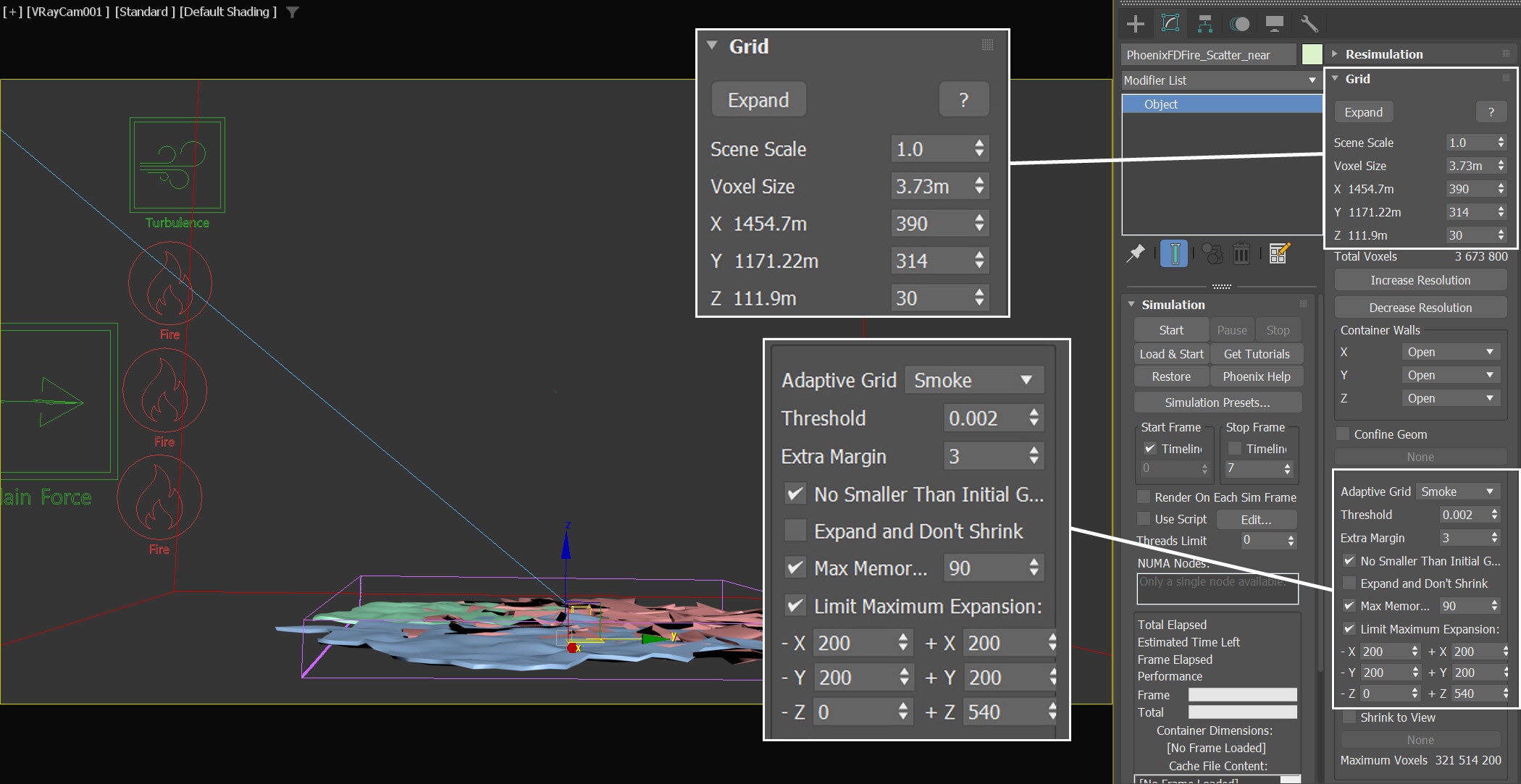
Here are the settings for the PhoenixFDFire_Scatter_near Simulator:
The exact position of the Phoenix Simulator in the scene is XYZ: [183.0, -63.0 -42.0].
Open the Grid rollout and set the following values:
- Voxel Size: 3.73 m
- Size XYZ: [390, 314, 30]
- Expand the Container Walls, so that they match the sizes of the Grid's X, Y and Z parameters
- Set the Adaptive Grid to Smoke. The Adaptive Grid algorithm allows the bounding box of the simulation to dynamically expand on-demand
- Set the Threshold to 0.02. This allows the simulator to expand when the Voxels near the corners of the simulation bounding box reach a Smoke value of 0.02 or greater
- Enable Maximum Expansion and set its parameters accordingly:
X: (200, 200)
Y: (200, 200)
Z: (0, 540)
This saves memory and simulation time by limiting the maximum size of the simulation grid.
The simulator has the Cloud_render_preset.tpr loaded, so the volumetric is all set for the final render.
Since this cloud will be duplicated through Chaos Scatter, we use relatively low grid resolution for the simulator to improve performance. However, since the cloud scatters near the camera, we need to make sure that the cloud has enough detail.
Select the Simulation rollout of the PhoenixFDFire_Scatter_near Simulator. We only need to simulate 7 frames, so set the Stop Frame to 7. Press the Start button to simulate.
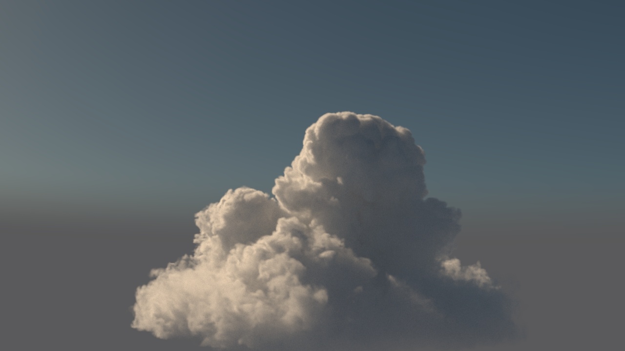
Run a test render of frame 7. This is our asset for the Cloud_for_scatter_near cloud.
Creating the Anvil Cloud
We created assets for all the cumulus clouds and can move on to creating another type of cloud.
To get started, open the Anvil_cloud_start.max scene. We have prepared a geometry, a camera, and a VraySun for you to use. An anvil cloud is essentially a cumulus cloud before it reaches the ceiling of the stratosphere, so we can apply the experience we gained from making the cumulus clouds to the anvil cloud. Therefore, we will skip some of the steps and focus more on the formation of the distinctive "anvil" shape of this cloud type.
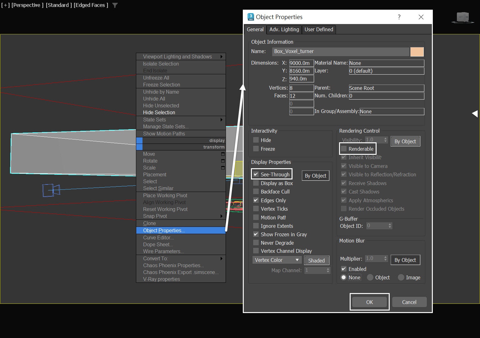
Compared to the setup for the Cumulus cloud, the Anvil cloud features one significant difference: a box that will be used in later steps to emulate the stratosphere. By incorporating this geometry together with a Voxel Tuner and a Plain Force, we can simulate horizontal cloud movement, ultimately achieving the distinctive anvil shape.
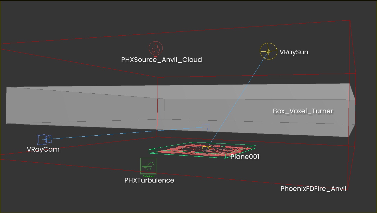
Rename the box to Box_Voxel_Tuner.
Set its Length, Width and Height to 8160.0m, 900.0m and 940.0m, respectively. Set the Segs for all axes to 1.
The exact position of the Box_Voxel_Tuner is XYZ: [125.0, -223.0, 808.0].
This box is used for defining the region of the Stratosphere where the cloud stops going up, and is blown to the side by a wind force. The position of the box allow us to create an anvil cloud with a height of 860 meters. This corresponds to the height of a real anvil cloud.
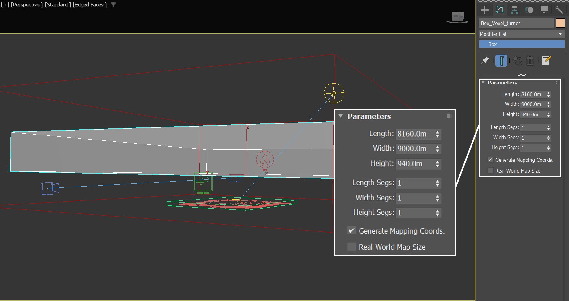
Since the Box_Voxel_Tuner is only used for the Voxel Tuner in a later step, we don't have to render the geometry. In its Object Properties, disable the Renderable checkbox and enable See-Through.
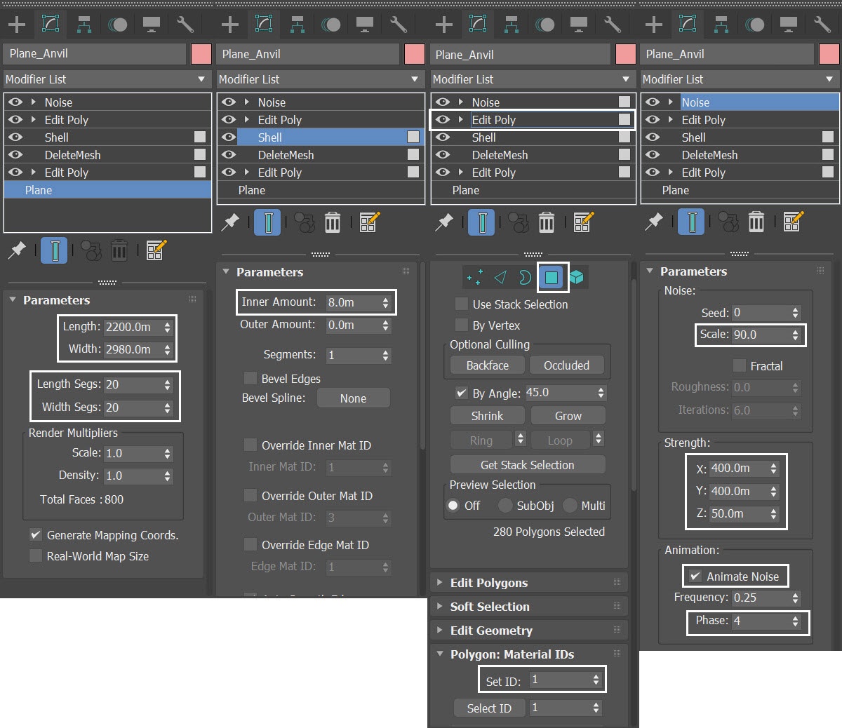
Several modifiers have been applied to the plane geometry, which uses the same settings as the planes for the Cumulus Cloud. To create the desired effect, the Phase of the Noise modifier is animated from a value of 1, at frame 0, up to a value of 4, at frame 15.
Note that 30% of the Plane_Anvil's faces got deleted, same as before, when we created the cumulus cloud assets.
Simulator for the Anvil Cloud
In the sample scene, we have set up a simulator for you. The simulator is named PhoenixFDFire_Anvil.
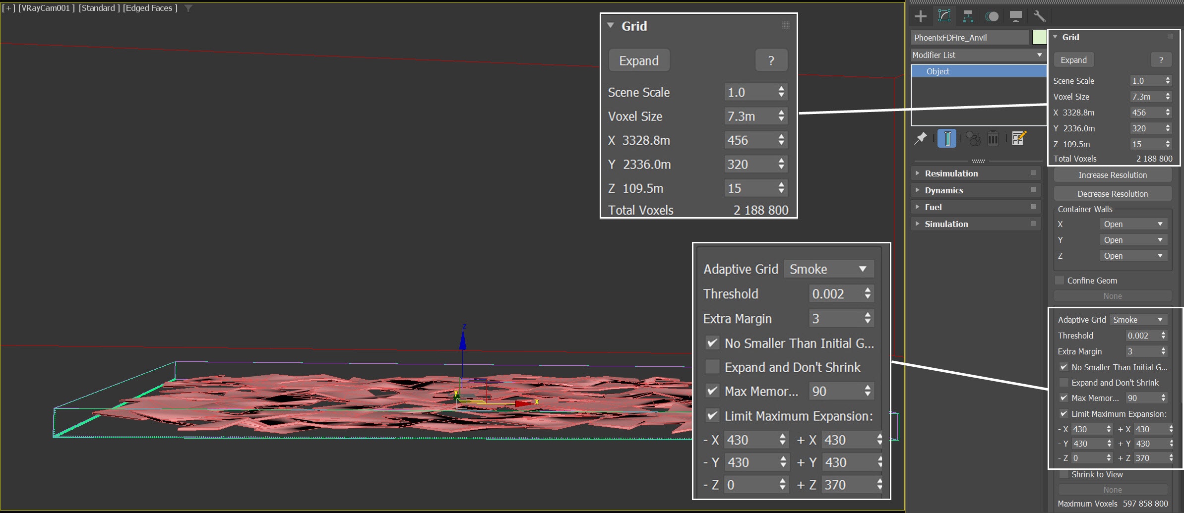
The exact position of the Phoenix Simulator in the scene is XYZ: [0.0, 0.0, -40.0].
Open the Grid rollout and set the following values:
- Voxel Size: 7.3 m
- Size XYZ: [456, 320, 15]
- Set the Adaptive Grid to Smoke. The Adaptive Grid algorithm allows the bounding box of the simulation to dynamically expand on-demand
- Set the Threshold to 0.02. This allows the simulator to expand, when the Voxels near the corners of the simulation bounding box reach a Smoke value of 0.02 or greater
- Enable Limit Maximum Expansion and set its parameters accordingly:
X: (430, 430)
Y: (430, 430)
Z: (0, 370)
This saves memory and simulation time by limiting the maximum size of the simulation grid.
The simulator is loaded along with the Cloud_render_preset.tpr, so the volumetric is all set for the final render.
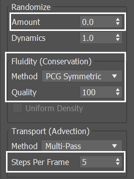
In the Dynamics rollout of the PhoenixFDFire_Anvil, we have set the Fluidity Method to PCG Symmetric and the Quality to 100. However, we have decided to lower the Steps Per Frame to 5 instead of 10.
Since the anvil cloud does not require as much detail as the cumulus cloud, we set the Steps Per Frame to 5 and leave the Randomize Amount at 0.0. Additionally, we keep the Noise for the source at 0.0.
Fire/Smoke Source for the Anvil Cloud
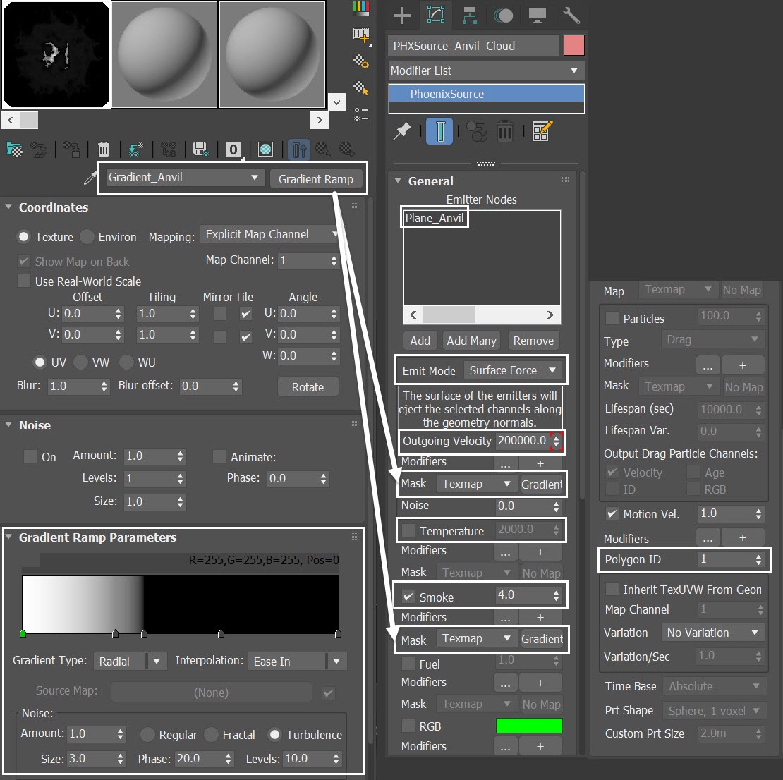
Set up the PHXSource_Anvil_Cloud's properties:
Set the Emit Mode to Surface Force
Disable the Temperature
Set the Smoke to 4.0
- Set the Outgoing Velocity Mask and Smoke Mask types to Texmap
Set the Polygon ID to 1. This limits the emission only to faces with an ID of 1
Create a Gradient Ramp:
- Plug the map into the Outgoing Velocity's and Smoke's Texmap slot
- Rename the map to Gradient_Anvil
- Set the Gradient Type to Radial. This produces a circular texture ideal for the base of the cloud
- Set the Noise parameters:
Set the Noise Amount to 1.0
Set the Size to 3.0
Set the Noise type to Turbulence
- Add 3 extra flags to the gradient bar, so that there are a total of 5
- Set the Interpolation to Ease Out
- Edit the positions of the five flags on the gradient map using the table
Flag | Position | RGB | Interpolation |
|---|---|---|---|
1 | 0 | 255,255,255 | Ease In |
2 | 29 | 68,68,68 | Ease In |
3 | 37 | 12, 12, 12 | Ease In |
4 | 63 | 1, 1, 1 | Ease In |
| 5 | 100 | 0, 0, 0 | Ease In |
Table of five flags on the gradient bar of the Gradient_Anvil . From left (start point) to right (end point).
Feel free to tweak this gradient map to create different cloud variants.
Changes to the Noise parameters greatly influence the simulated cloud. It is recommended that you experiment with different settings once you've completed this tutorial. If you want to recreate the same result as shown here, follow the instructions exactly.
Please note that it is important to mask both the Outgoing Velocity and the Smoke in the source, to achieve a distinct anvil-shaped cloud. We recommend doubling the Smoke amount from a value of 2.0 to a value of 4.0.
Animation of the Outgoing Velocity of the Anvil Cloud
- Go to Graph Editors > Track View - Curve Editor
- Set keyframes for the Outgoing Velocity for PHXSource_Anvil_Cloud, so it can change over time. Each frame and value is shown in the screenshot and in the table
Frame | Value | Tangent type |
|---|---|---|
0 | 200000.0 | Fast |
5 | 0.0 | Slow |
Keyframes for the FIre/Smoke Source's Outgoing Velocity
Please note that the Tangent type is crucial for achieving the desired anvil shape. To ensure the correct settings, please refer to the table provided.
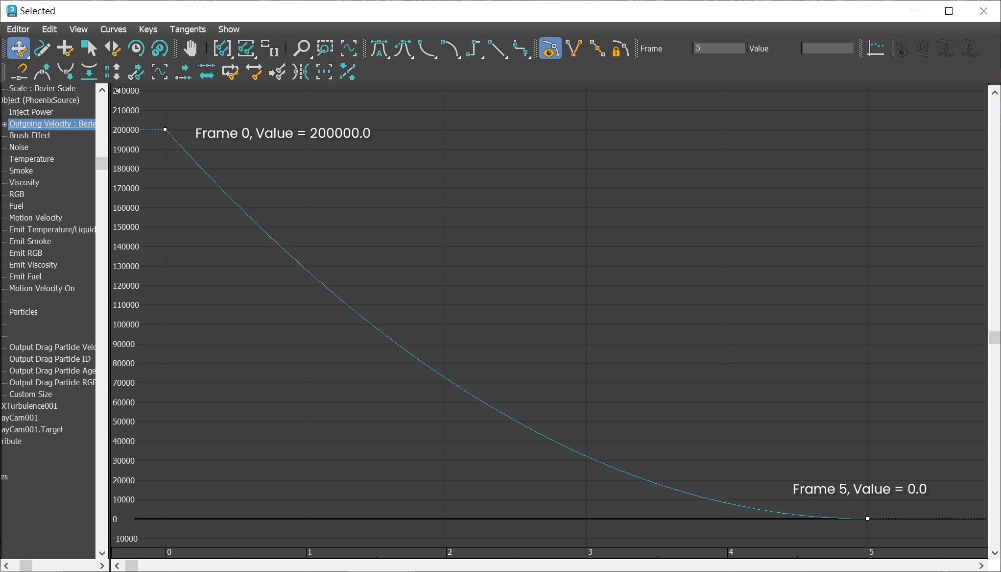
Screenshot of the Outgoing Velocity keyframes
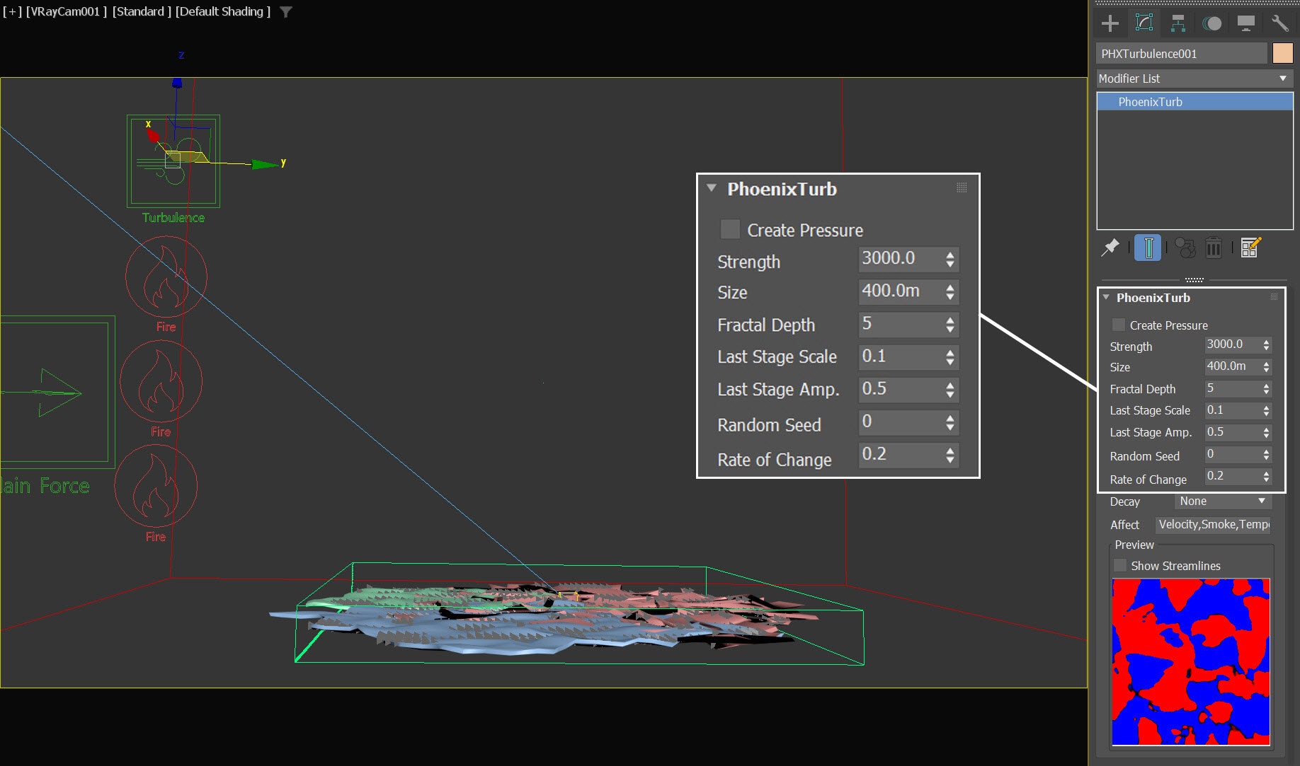
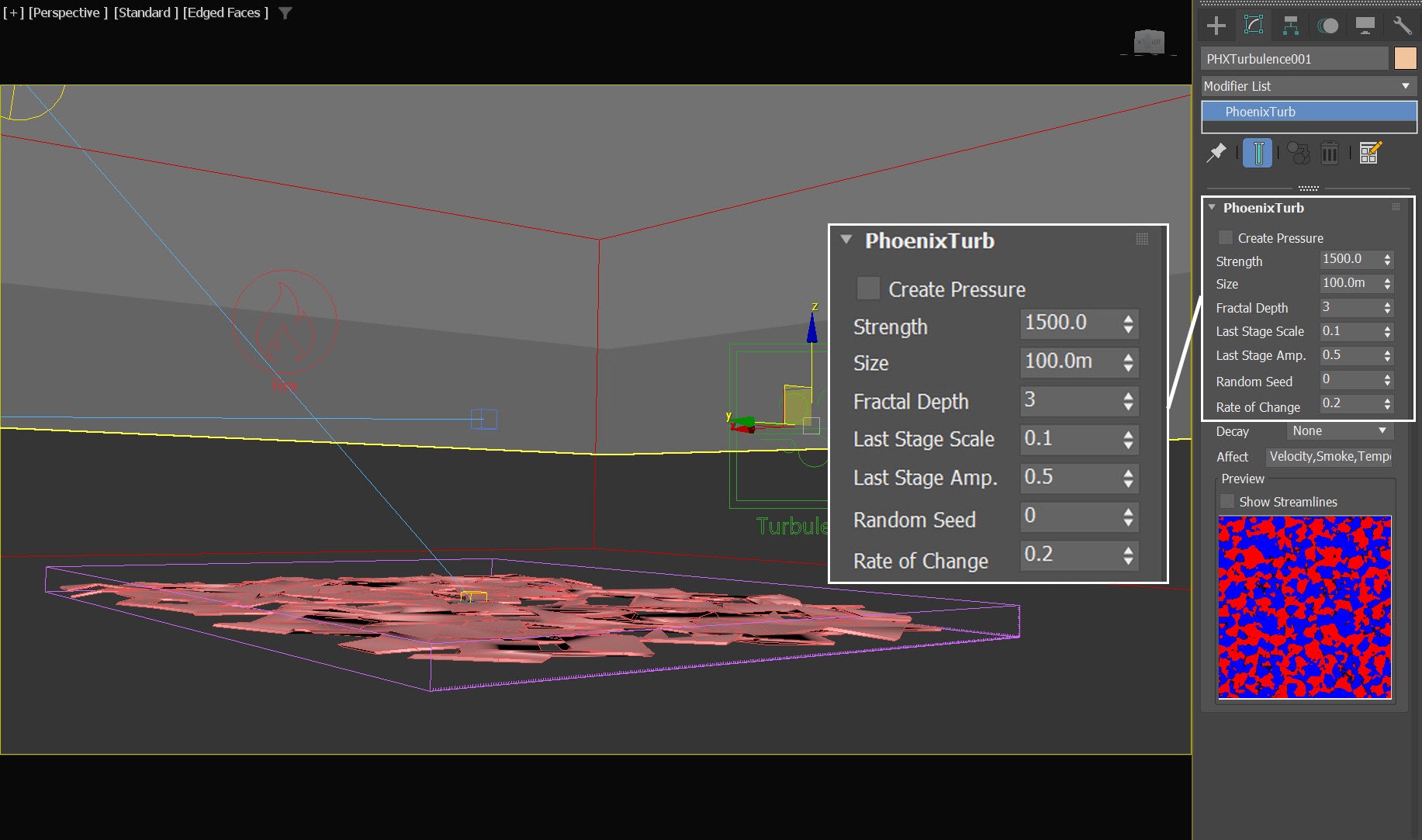
Settings for the Phoenix Turbulence
Apply the same PHXTurbulence settings as the ones in the Cumulus_A scene. Here are the details:
- Set the position to XYZ: [ -1769.0, 1200.0, 630.0]
- Set the Strength to 1500.0
- Set the Size to 100.0m
- Set the Fractal Depth to 3
- Reduce the Rate of Change to 0.2
Initial Simulation of the Anvil Cloud
Select the Simulation rollout of the PhoenixFDFire_Anvil Simulator. We only need to simulate 11 frames, so set the Stop Frame to 11. Press the Start button to simulate.
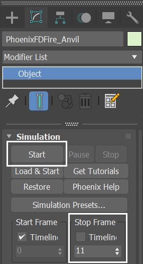
This voxel preview shows the current animation. You can see a mushroom-like shape. Additional procedures are needed to achieve the distinctive "anvil" shape of this cloud type.
Adding Plain Force
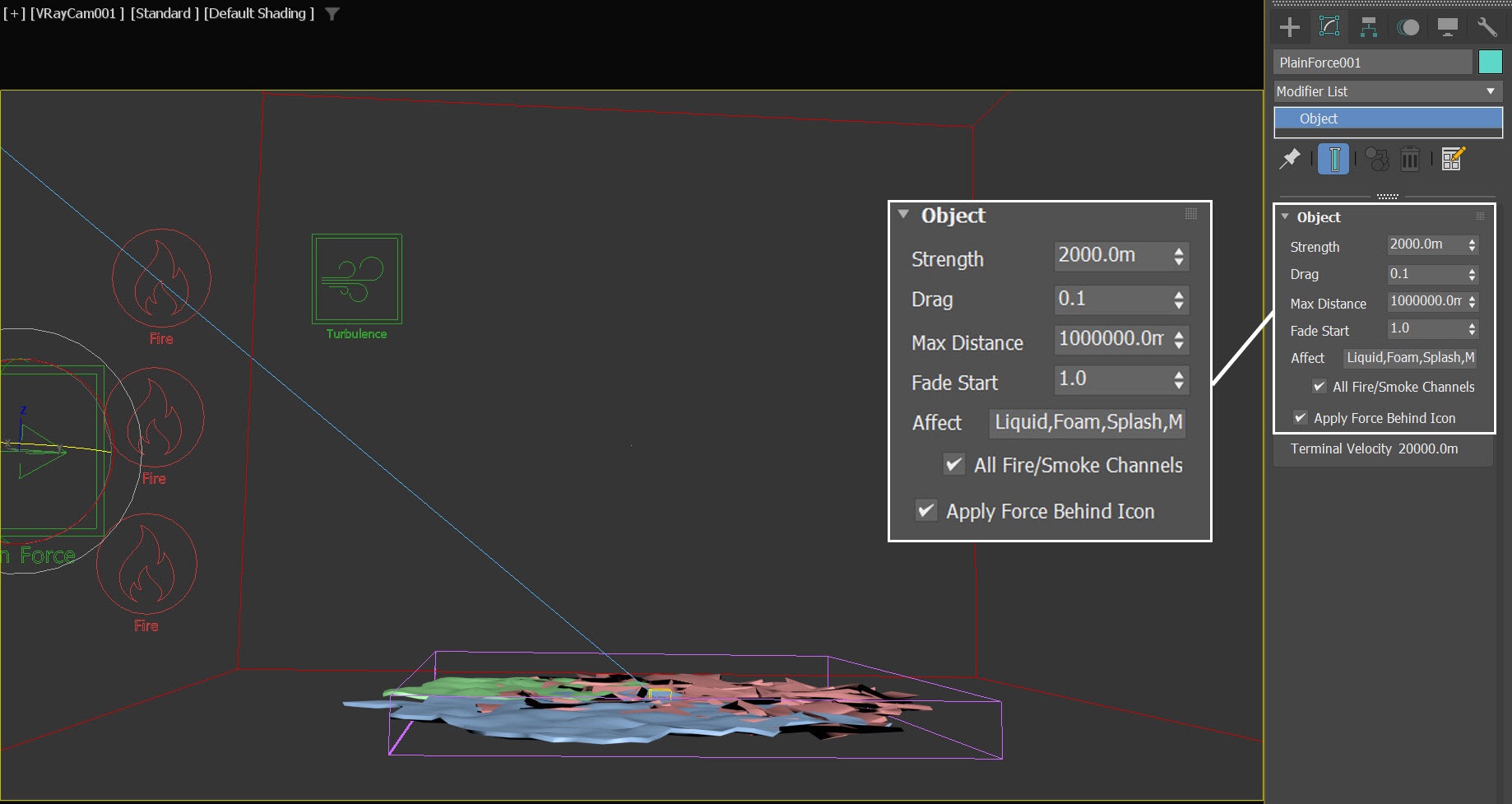
To replicate the atmospheric conditions of the Stratosphere, we can introduce a Phoenix Plain Force into the scene. To do this, go to Create Panel > Helpers > Phoenix and add a Phoenix Plain Force.
The exact position of the Plain Force in the scene is XYZ: [1867.0, 0.0, 486.0]
Set the Strength to 2000.0m
Set the Drag to 0.1
Enable the Apply Force Behind Icon option
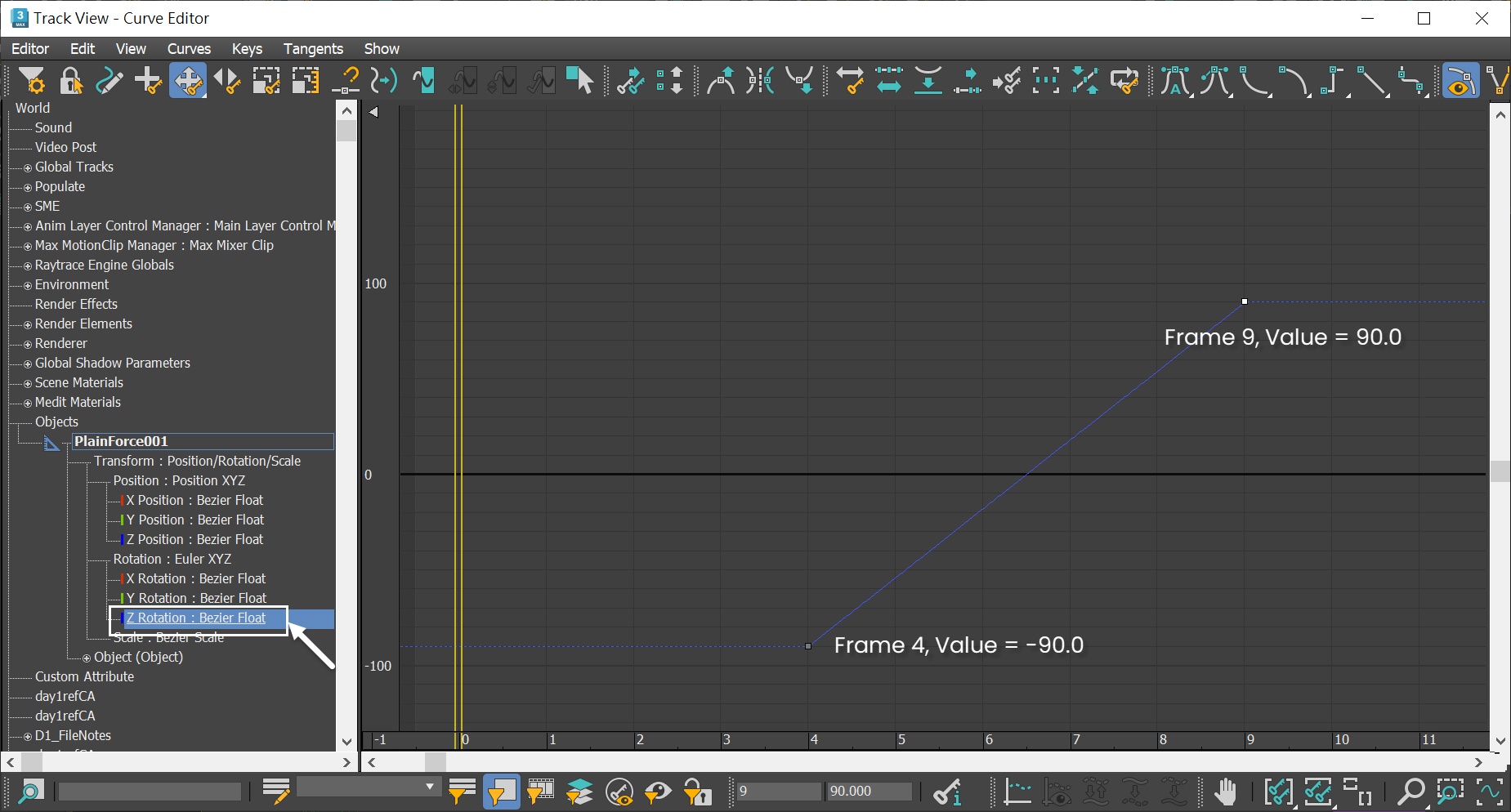
To make the visual effect more interesting, animate the Plain Force. Refer to the screenshot for the appropriate frame numbers and values. Set all tangents to Linear.
Emulate the Stratosphere with a Particle Tuner and a Plain Force
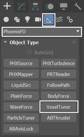
Go to Create Panel → Helpers → PhoenixFD → VoxelTuner. Create a Voxel Tuner anywhere in the scene.
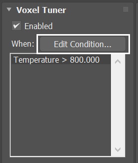
With the Voxel Tuner selected, click on the Edit Condition button to change the condition.
The Voxel Tuner assesses all voxels in the simulation and, under a given condition, changes their values.
In this example we limit the Plain Force to only affect the designated region - inside of Box_Voxel_Turner.
The conditions can be very simple, but you can also build more complex conditions with the Voxel Tuner's Expression operators.
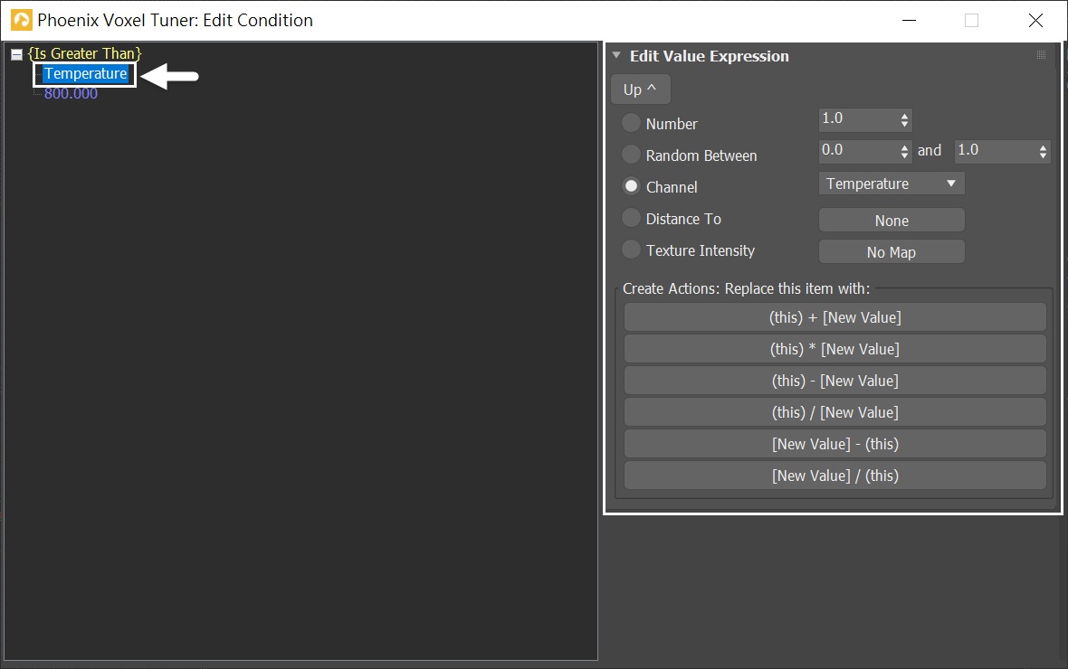
In the Edit Condition window, click on Temperature. The Edit Value Expression window shows up.
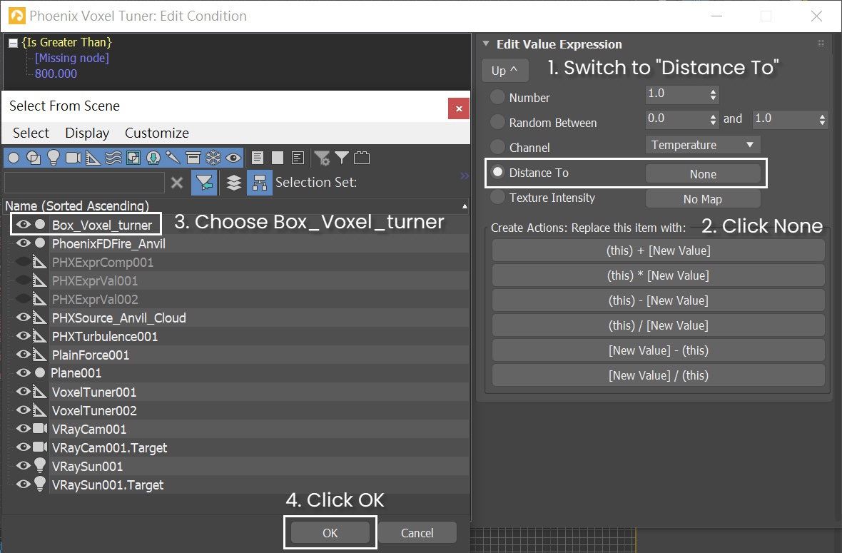
Switch the condition from Channel - Temperature to Distance To. Press the None button and choose the Box_Voxel_Turner geometry from the scene.
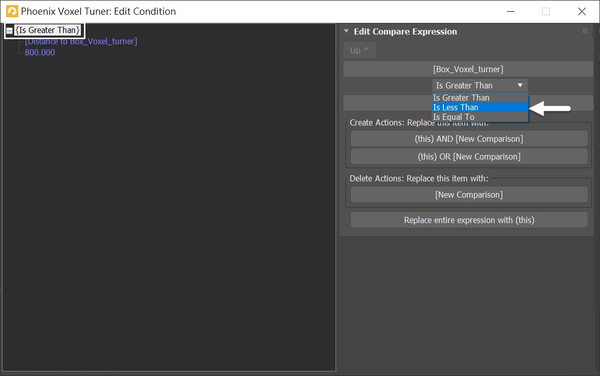
Click on the Is Greater Than condition, so the Edit Compare Expression window shows on the right. Change the condition from Is Greater Than to Is Less Than.
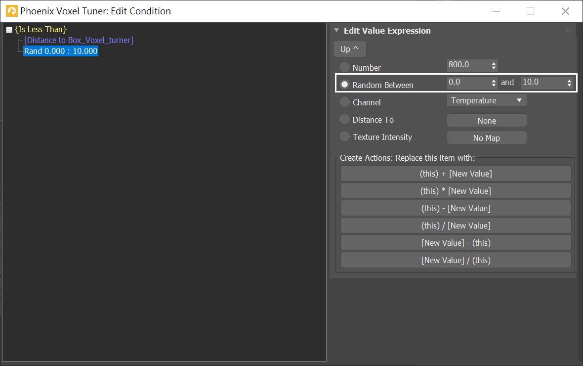
Click on the value of 800.0, change the Value Expresion to Random Between. Edit the value so you have random value from 0.0 to 10.0
Note that the unit for distance in the Voxel Tuner is in simulation grid voxels. If you change the simulator's Grid Resolution, this also changes the units that the Voxel Tuner uses to measure distance.
The distance to the box is randomized between 0.0 to 10.0, allowing us to simulate a cloud with a softer and more natural anvil top. You can adjust this value to fit your preference.
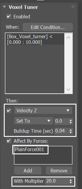
After configuring the condition settings, close the Edit Condition window. Next, change the Then parameter to Velocity Z. Set the value to 0.0 and adjust the Buildup Time (sec) to 0.04.
To add a force to the scene, go to Affect By Forces and click on the Add button. Select the PlainForce.
For the anvil shape, a strong wind force is needed. To increase the effect, adjust the With Multiplier parameter to 20.0.
This is the condition set by the Voxel Tuner: when the cloud is near or inside the Box_Voxel_Tuner region, it stops moving upward and is pushed by the PlainForce.
To achieve a gradual transition of the effect, we introduce a one-frame delay. Given that our animation runs at 30 frames per second, the delay time is approximately 0.03333 seconds, or rounded to 0.04 seconds. Feel free to adjust this value to your liking.
With those new settings, run the simulation again.
This voxel preview shows the current animation. Now we see the cloud forming an anvil shape.
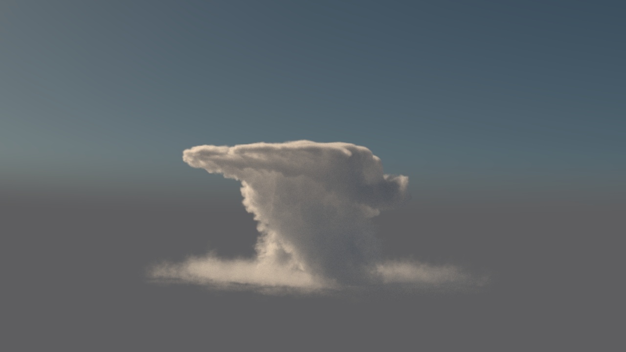
Run a test render of frame 11. This is our asset for the Anvil_cloud.
We stopped at frame 11 to achieve a subtle anvil-shape look for the cloud. Simulating for longer would create a more dramatic effect, which would be less realistic.
Creating the Stratus_top Cloud
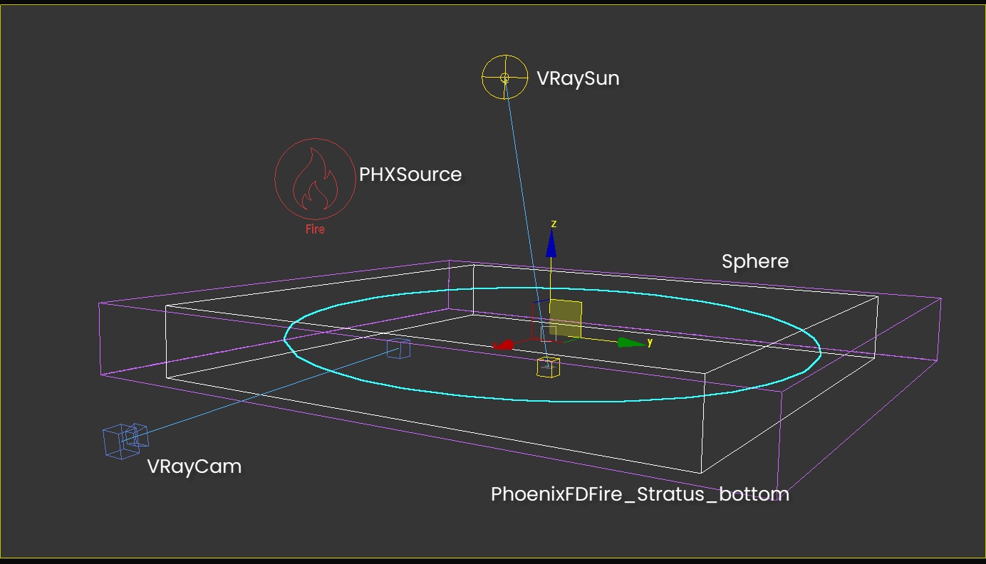
To start, let's open the file "Startus_top_start.max" which includes a VRaySun, a VRay Camera, and a Sphere.
The sphere has a diameter of 3244.0 meters and 32 segments. It's been flattened and scaled down to 13% of its original height along the Z-axis.
Smoke is going to be emitted from this sphere. Flattening it will create a flat stratus cloud. To customize the height of the cloud, adjust the sphere's size along the Z-axis.
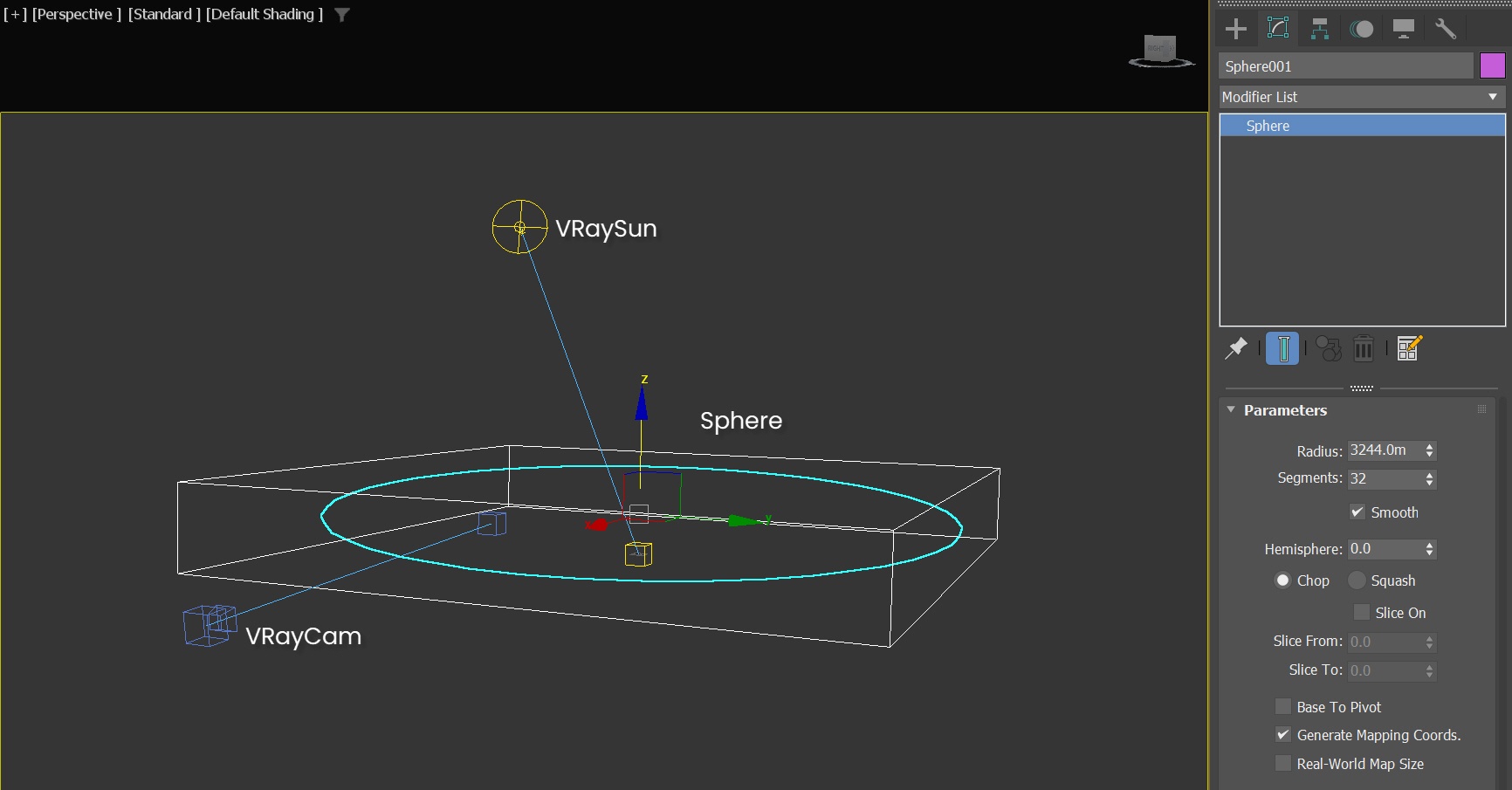
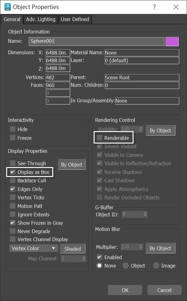
Since the sphere is used solely as a smoke source, the Renderable checkbox is disabled and Display as Box is enabled in its Object Properties.
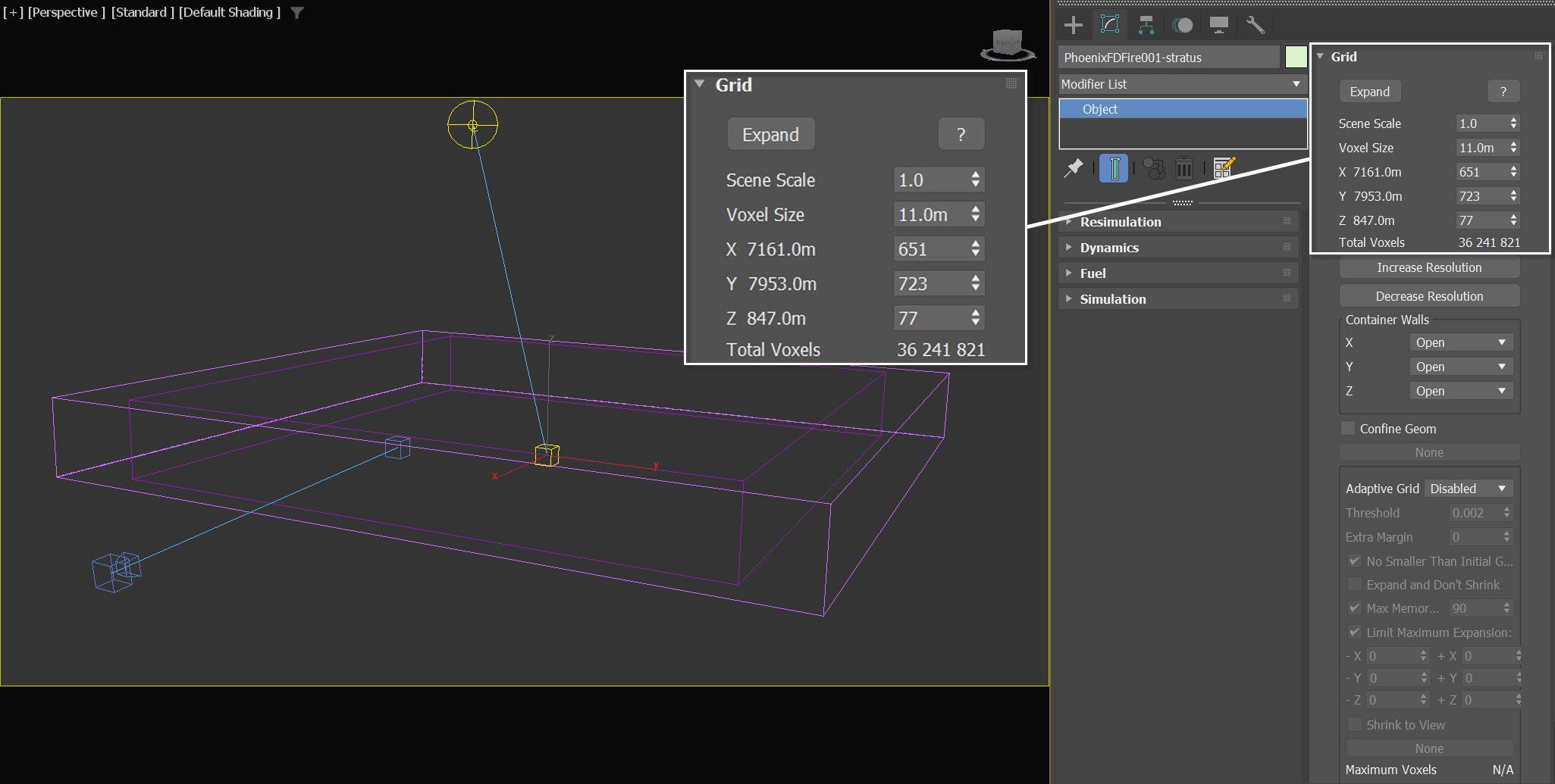
Go to Create Panel > Create > Geometry > PhoenixFD and click on FireSmokeSim. Rename the simulator to PhoenixFDFire_Stratus_top.
Position it in the scene at XYZ: [0.0, 0.0, 0.0]
Open its Grid rollout and set the following values:
Voxel Size: 11.0 m
- Size XYZ: [ 651, 723, 73 ]
Open the Container Walls to match the X, Y and Z of the Grid Size
Adding a Fire/Smoke Source for the Stratus Cloud
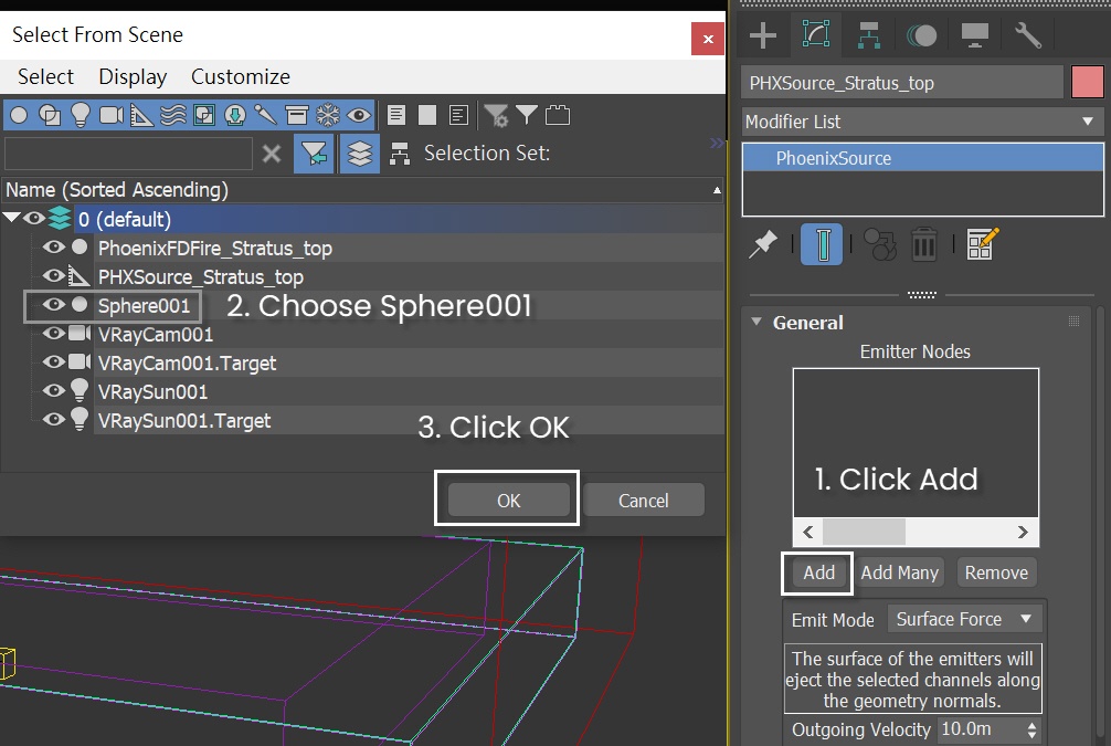
Go to the Create Panel > Create > Helpers > PhoenixFD and create a PHXSource. Rename it to PHXSource_Stratus_top.
Press the Add button to choose which geometry to emit from and select the Sphere001 in the Scene Explorer.
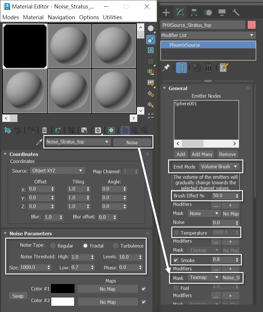
PHXSource_Stratus_top settings:
- Set the Emit Mode to Volume Brush
- Set the Brush Effect % to 50.0
- Disable the Temperature option
- Set the Smoke to 0.8
- Set the Smoke Mask to Texmap and plug a Noise texture map into the slot and rename it to Noise_Stratus_top.
Set the Size to 1000.0
Set the Hight to 1.0
Set the Low to 0.7
Set the Noise Type to Fractal
Set the Levels to 10.0
To create a thinner layer of stratus cloud that intersects with the cumulus clouds, we set a low Smoke value of 0.8.
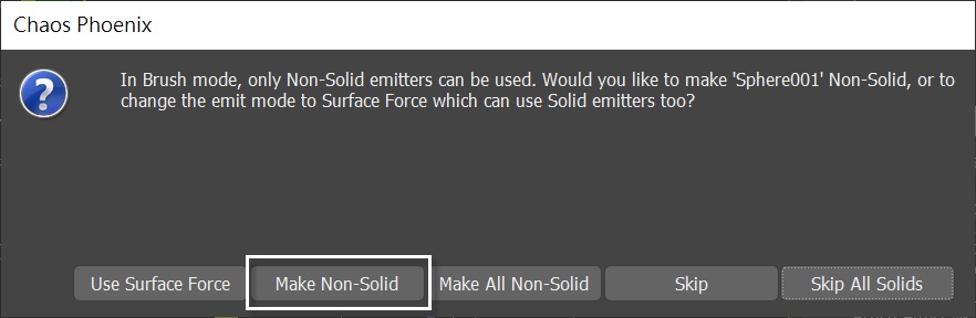
When switching the Emit Mode to Volume Brush, Phoenix prompts you to make the Sphere001 non-solid. Click on Make Non-Solid. Otherwise, it collides with the fluid simulation.
Unlike the cumulus cloud, the stratus cloud doesn't need to have great details, so leave everything in the Dynamics rollout at its default.
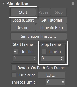
Select the Simulation rollout of the PhoenixFDFire_Stratus_top Simulator. We only need to simulate 3 frames, so set the Stop Frame to 3. Press the Start button to simulate.
With the PhoenixFDFire_Stratus_top selected, go to the Rendering rollout. Click on the Render Presets and click on Load from File. Load the Cloud_render_preset.tpr, provided with the sample scene.
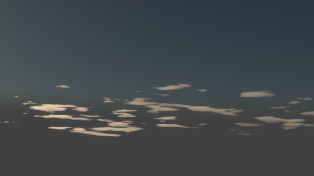
Run a test render of frame 3. This is our asset for the Stratus_top cloud.
Creating the Stratus_bottom Cloud
The Startus_bottom has basically the same setup, so we don't need to repeat the procedure. Open up the final scene "Startus_bottom_final.max". It already has the Phoenix Source and Simulator set up for you. The simulator is renamed to PhoenixFDFire_Startus_bottom.
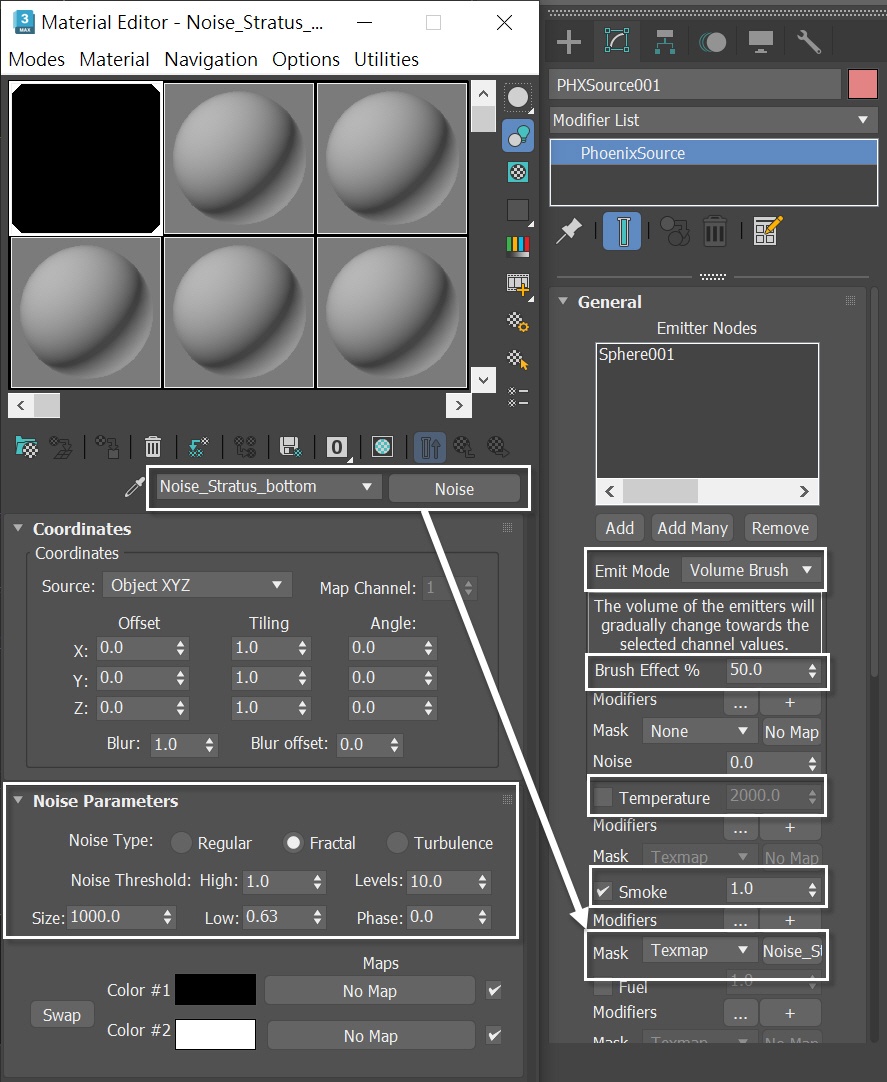
Here are the settings for PHXSource_Stratus_bottom:
- Set the Smoke to 1.0
- Set the Smoke Mask to Texmap and plug a Noise texture map into the slot. Rename the map to Noise_Stratus_bottom.
Set its Size to 1000.0
Set its High to 1.0
Set its Low to 0.63
Set its Noise Type to Fractal
Set its Levels to 10.0
Setting the smoke to 1.0 creates a thicker stratus cloud, and lowering the value of the Low Noise Threshold increases the area the cloud covers. If the value of Low Noise is higher, it results in less area covered by the cloud.
Select the Simulation rollout of the PhoenixFDFire_Stratus_bottom Simulator. We only need to simulate a single frame, so set the Stop Frame to 1. Press the Start button to simulate.
Run a test render of frame 1. This is our asset for the Stratus_bottom cloud.
Scene Assembly
Assembling the Daytime Cloudscape
With all the volumetric data for the clouds ready, it's time to assemble them into a cloudscape. Open up the provided scene "Cloudscape_daytime_start.max". To help you get started, the scene includes an animated camera, a VRaySun, and some splines that will be used to scatter the VrayVolumeGrid. The scene also includes Omni lights, two PFLows, and one PCloud for the stormy night.
All the Omni lights, PFlows and the PCloud are hidden, as these elements are intended for the stormy night cloudscape. We will unhide them in a later step.
Alternatively, you can quickly assemble all the necessary cloud volumetric data by downloading them from the Phoenix Cloud Assets page.
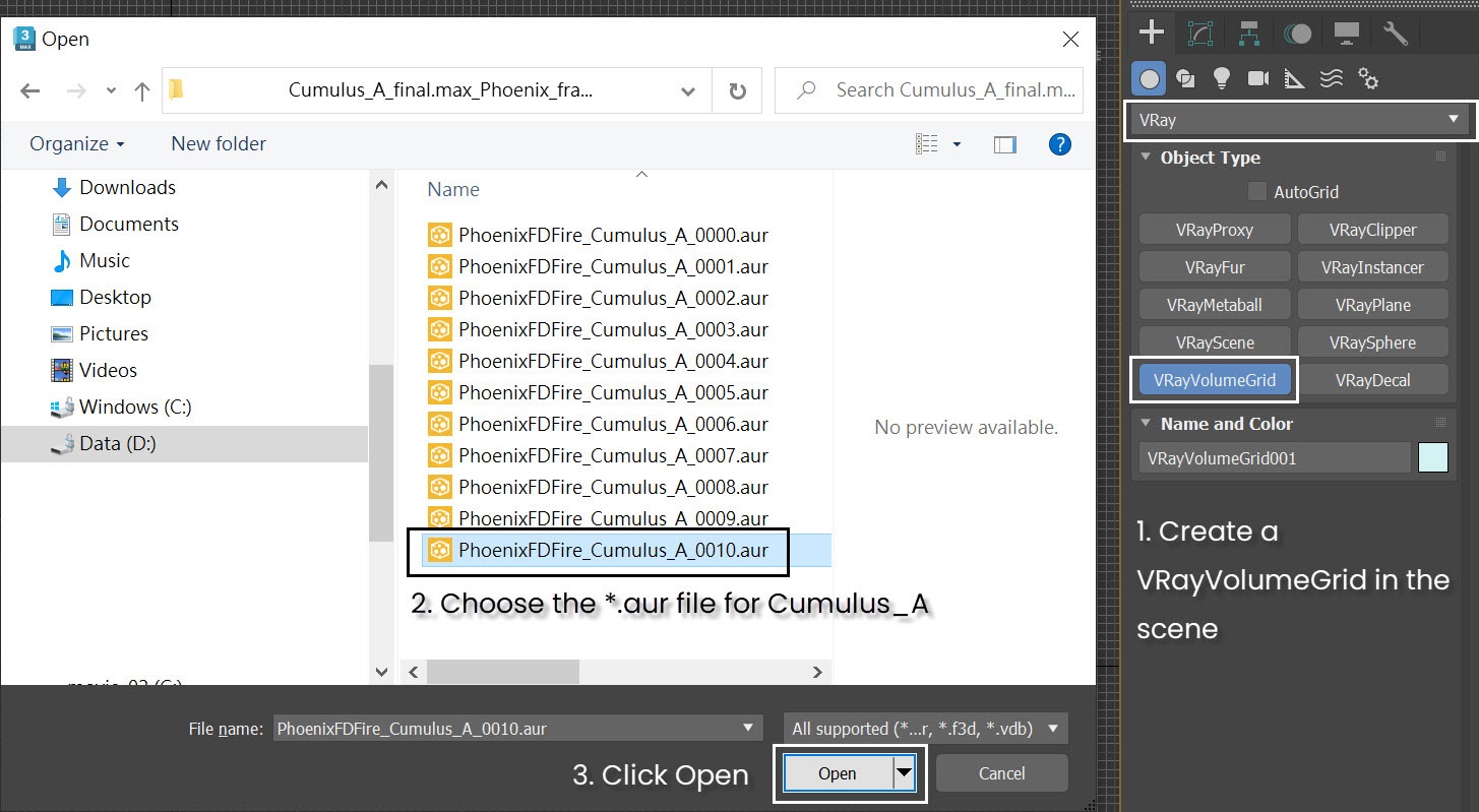
Go to Create panel > V-Ray. Click on the VRayVolumeGrid button and click anywhere in the scene. This prompts a dialog window. Locate the *.aur file for Cumulus_A. Open the file to load the cache into VRayVolumeGrid.
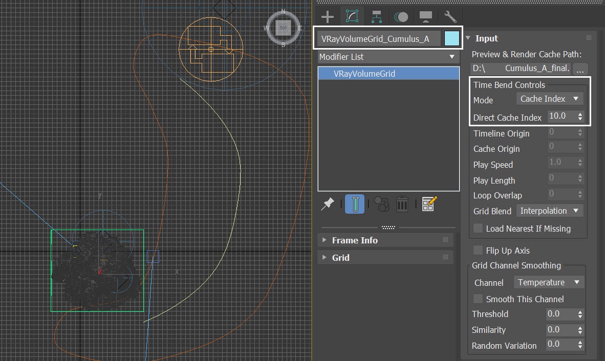
Rename the VRayVolumeGrid to VRayVolumeGrid_Cumulus_A. In the Input rollout, change Time Bend Controls Mode to Cache Index. Set the Direct Cache Index to 10.0.
With the VRayVolumeGrid_Cumulus_A selected, move it to XYZ: [183.0, -88.0, 0.0]. Rotate it to XYZ: [0.0, 0.0, -92.0].
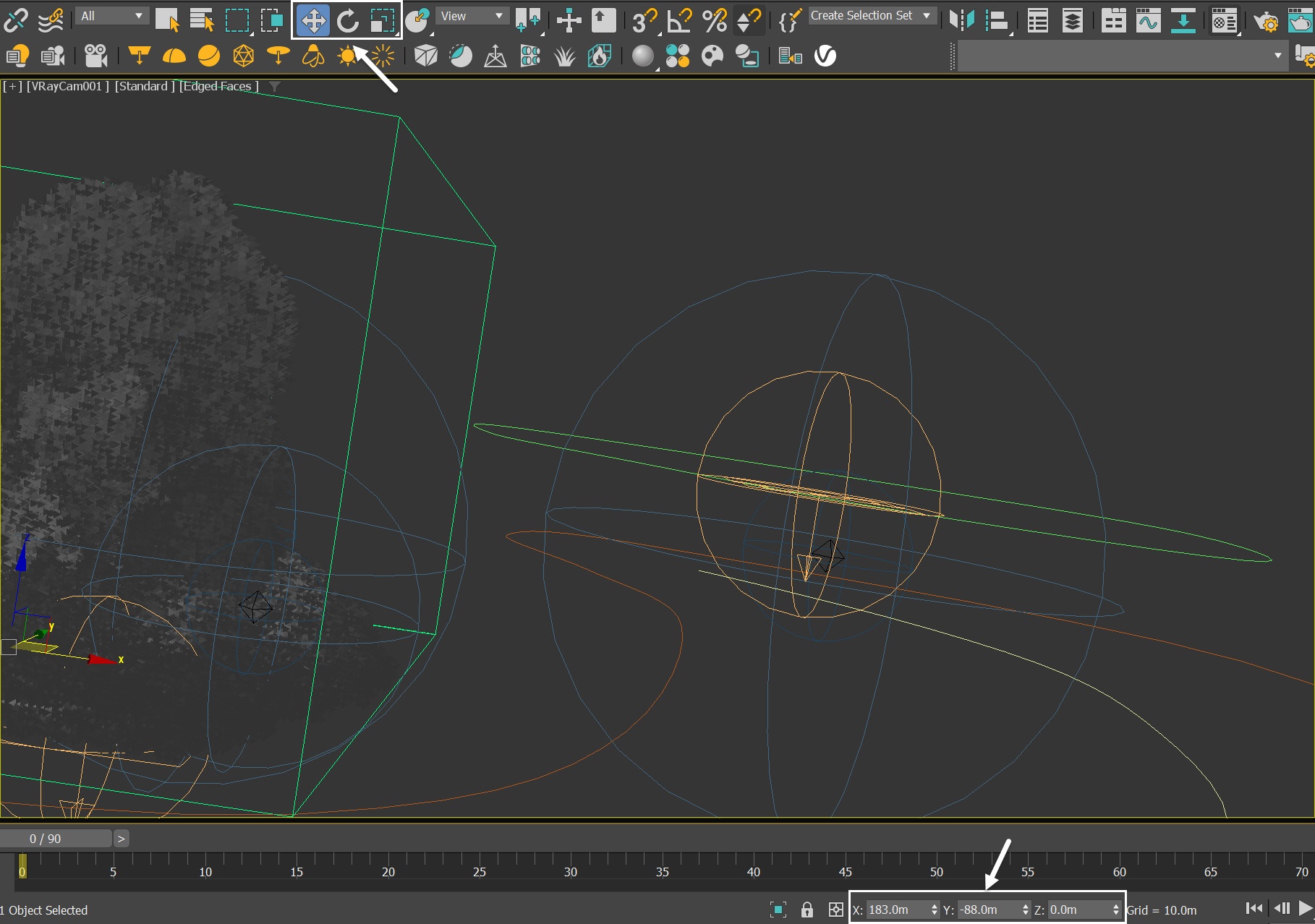
With the VRayVolumeGrid_Cumulus_A selected, go to the Rendering rollout. Click on Render Presets and select Load from File. Load the Cloud_render_preset.tpr that is provided with the sample scene.
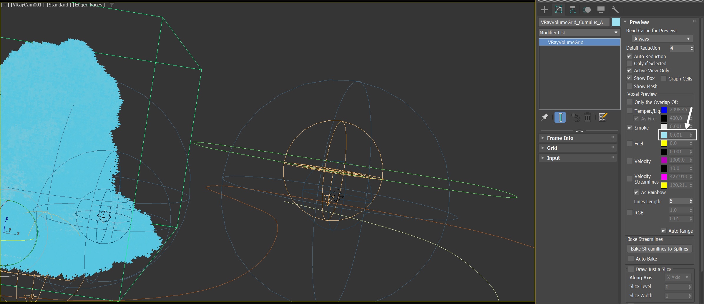
Go to the Preview rollout of the VRayVolumeGrid_Cumulus_A, change the color of the lowest smoke grid value to light blue - RGB(88,199,225).
Since the scene will contain many VRayVolumeGrids, each with a different cloud asset, changing their preview color would aid in distinguishing them.
Be sure to enable the Auto Reduction option in the Preview rollout, as we will be incorporating multiple VRayVolumeGrids into the scene. If you skip this step, it could cause a low viewport frame rate.
Great, we have successfully set up VRayVolumeGrid_Cumulus_A. However, there are six more cloud assets waiting to be loaded into the scene. Please follow the same procedure for each of the remaining cloud assets.
Scaling (82, 82, 82) means uniformly scaling down the VRayVolumeGrid to 82%.
Feel free to customize your cloudscape by adjusting the position, rotation, scale, or Direct Cache Index of each VRayVolumeGrid according to your preferences.
Position | Rotation | Scale | Direct Cache Index | Smoke preview color | |
|---|---|---|---|---|---|
Cumulus_A | 183.0, -88.0,0.0 | 0.0, 0.0, -92 | 100, 100, 100 | 10.0 | 88, 199, 225 |
Cumulus_B | 798, -737, 0 | 0, 0, -31 | 82, 82, 82 | 7.0 | 223, 86, 86 |
Anvil_cloud | 2842, 4554, 0 | 0, 0, 110 | 172, 172, 172 | 11.0 | 181, 51, 255 |
Cloud_for_scatter_near | 2880.0, 1076.0, 0.0 | 0.0, 0.0, 0.0 | 100, 100, 100 | 7.0 | 255, 143, 86 |
Cloud_for_scatter_far | 1688, 19677, 0 | 0, 0, 0 | 100, 100, 100 | 4.0 | 225, 86, 143 |
Stratus_top | 1492, 2862, 48 | 0 ,0 , -160 | 114, 114, 114 | 2.0 | 88, 88, 225 |
Stratus_bottom | 1942, 896, -840 | 0, 0, -132 | 128, 128, 128 | 1.0 | 5, 0, 229 |
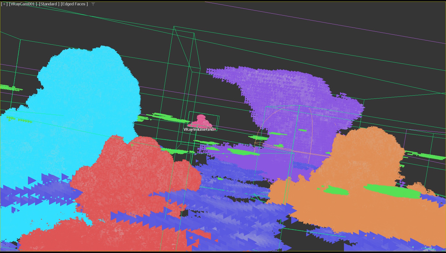
Now we have loaded all seven cloud assets into the scene with their VRayVolumeGrids. While it might look good, there are still many gaps in the frame that need to be filled. Otherwise, the cloudscape won't be convincing enough.
Scattering the Clouds with Chaos Scatter
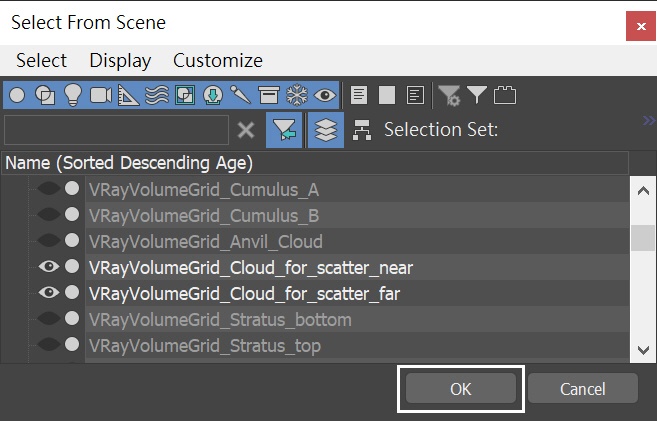
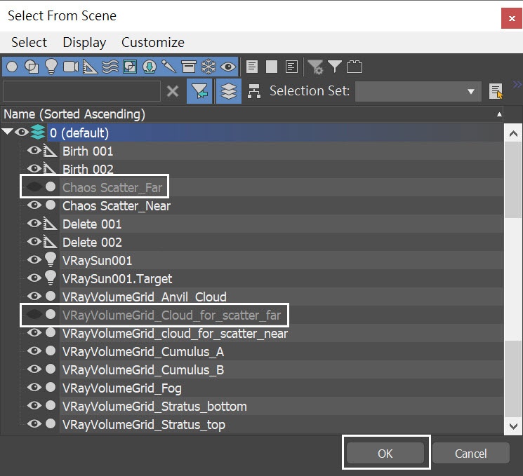
Before we apply Chaos Scatter to the cloud assets, let's simplify our workspace by hiding the other VRayVolumeGrids. To do this, open the Select by Name window and hide all VRayVolumeGrids, except for VRayVolumeGrid_Cloud_for_scatter_far and VRayVolumeGrid_Cloud_for_scatter_near, which are the ones we'll be working with.
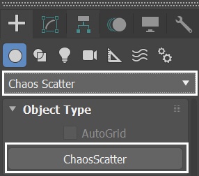
Navigate to the Create panel and select the Geometry tab. From the drop-down menu, select Chaos Scatter and create two Chaos Scatter geometries in the scene. To keep things organized, rename them as Chaos Scatter_Far and Chaos Scatter_Near, to match their respective purposes.
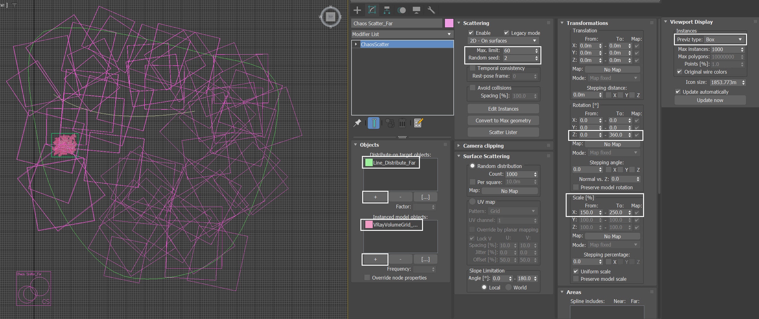
With the Chaos Scatter_Far selected, in the Objects rollout, use the "+" button to add Line_Distribute_Far to the Distribute-on target objects list. Then add the VRayVolumeGrid_Cloud_for_scatter_far to the Instanced model objects list. By doing this, the Cloud_for_scatter_far asset will be scattered within the enclosed region defined by the spline shape of Line_Distribute_Far.
- In the Scattering rollout, set the Max. limit to 60 and the Random seed to 2.
- In the Rotation section of the Transformations rollout, set the Z Rotation To to 360.0.
- In the Scale[%] section, set X From and To to 150.0 and 250.0, respectively.
- In the Viewport Display rollout, set the Previz type to Box.
The clouds in the distance do not require a high grid resolution, which is why we generate the VRayVolumeGrid_Cloud_for_scatter_far with a larger voxel size than the one for the close-up clouds.
To create a more diverse cloudscape, you can add multiple VRayVolumeGrids to the instanced model objects list. However, keep in mind that this may impact performance, so for this tutorial, we will only be using one.
The Previz type is temporarily set to Box. This makes it easier to check the dimensions of the scattered cloud. Once we finalize the settings, you can switch the Previz type to Dot, which won't obstruct the view of other objects in the cloudscape.
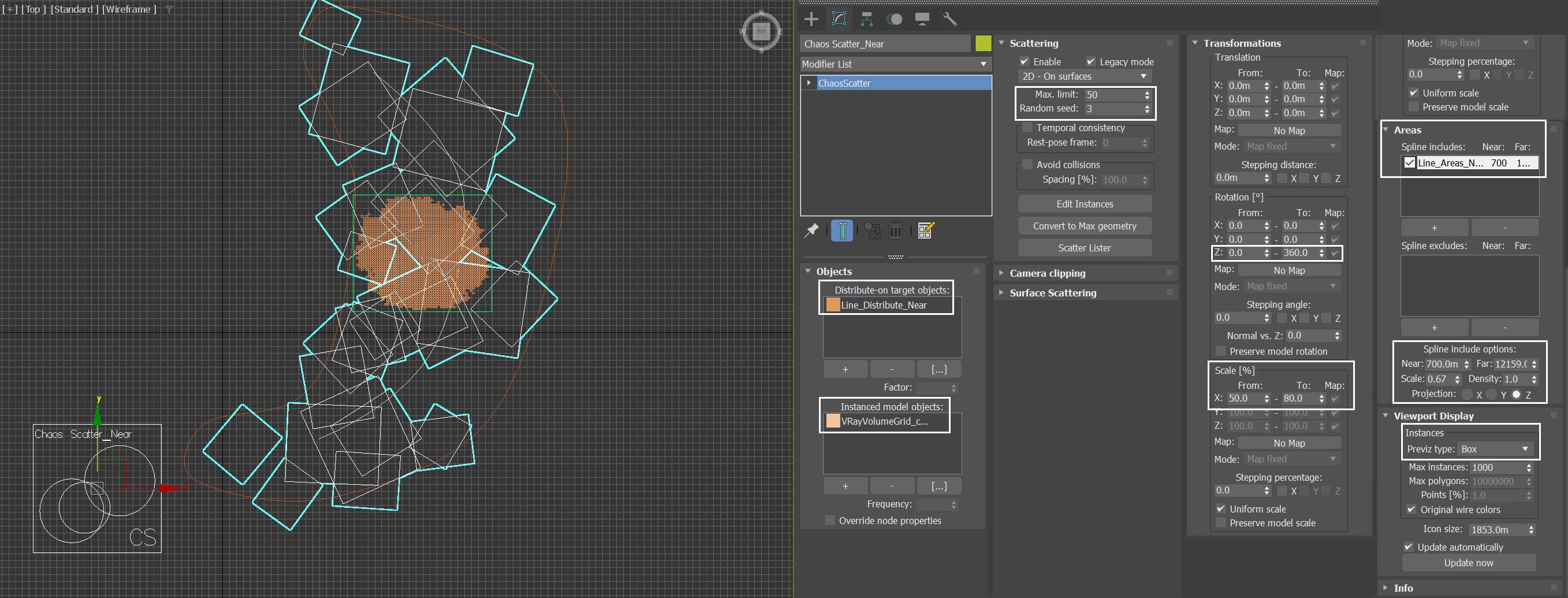
With the Chaos Scatter_Near selected, in the Objects rollout, use the "+" button to add Line_Distribute_Near to the Distribute-on target objects list. Then add the VRayVolumeGrid_Cloud_for_scatter_near to the Instanced model objects list. By doing this, the Cloud_for_scatter_near asset will be scattered within the enclosed region defined by the spline shape of Line_Distribute_near.
- In the Scattering rollout, set the Max. limit to 50 and the Random seed to 3.
- In the Rotation section of the Transformations rollout, set the Z Rotation To to 360.0.
- In the Scale[%] section, set X From and To to 50.0 and 80.0, respectively.
- In the Areas rollout, add Line_Areas_Near to the Spline includes list. Click on the item and set the Near distance to 700.0m and the Far distance to 12159.0m. Finally, set the Scale to 0.67 and the Density to 1.0.
- In the Viewport Display rollout, set the Previz type to Box.
The spline in the Areas rollout allows you to create smaller clouds that are far away from the specified spline, and larger ones that are near it. This provides a more natural distribution and size of the clouds.
The Previz type is temporarily set to Box. This makes it easier to check the dimensions of the scattered cloud. Once we finalize the settings, you can switch the Previz type to Dot, which won't obstruct the view of other objects in the cloudscape.
Creating Fog Using VRayVolumeGrid
Unhide all VRayVolumeGrids in the scene.
Now we have all the clouds set for a cloudscape, but we still need something for a better aerial perspective - fog.
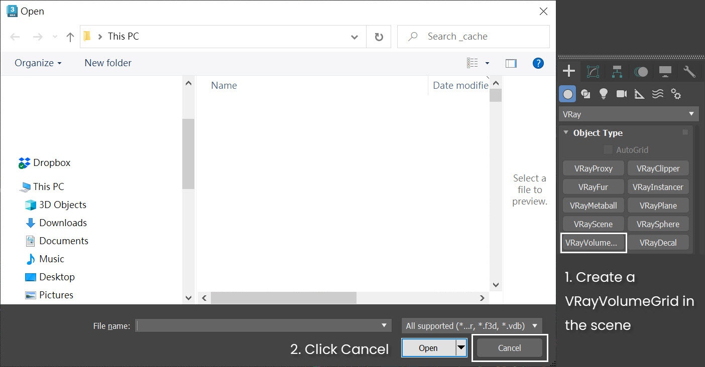
Go to Create panel > V-Ray. Click on the VRayVolumeGrid button and click anywhere in the scene. This prompts a dialog box for loading cache files. Click on Cancel.
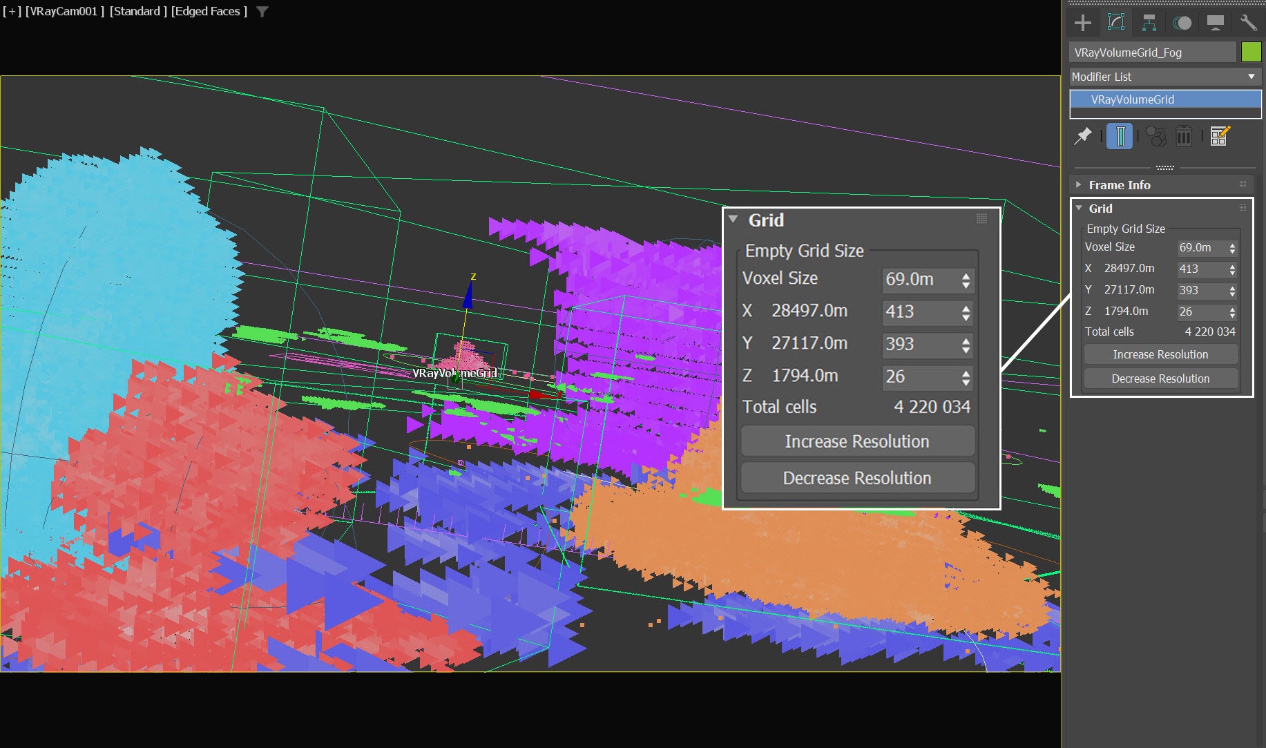
Rename the VrayVolumeGrid we just created to VRayVolumeGrid_Fog. Move it to XYZ: [1452.0, 14455.0, 0.0].
In the Grid rollout, set the following settings:
- Voxel Size: 69.0m
- Size XYZ: [413, 393, 26]
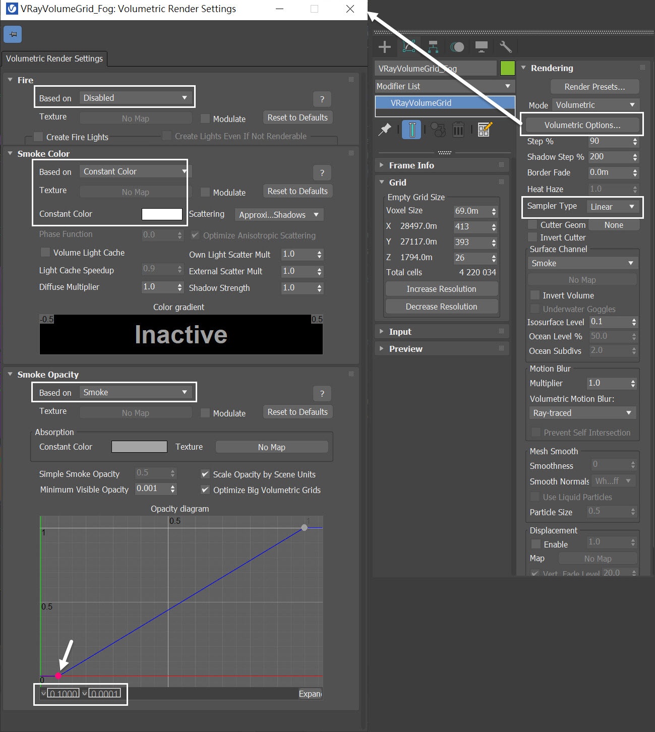
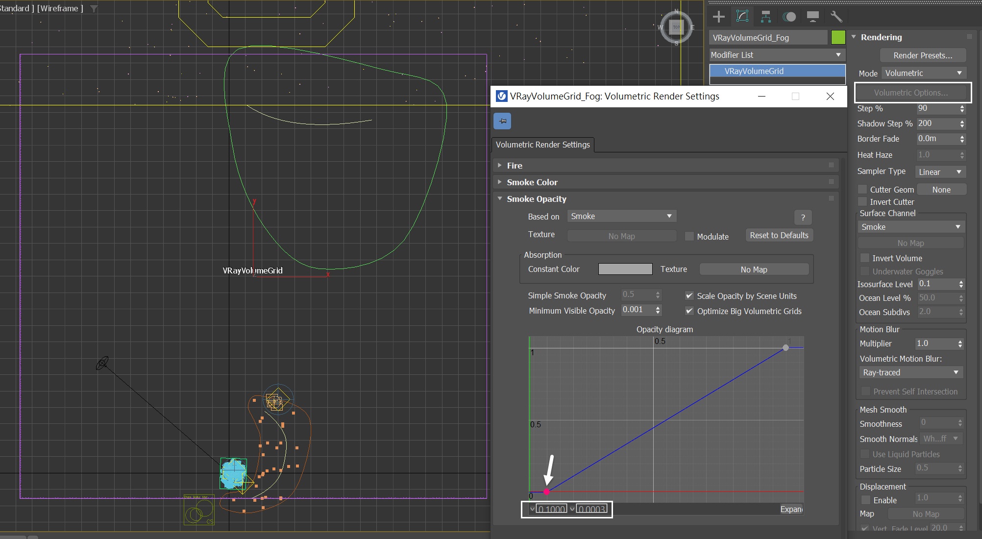
Select VRayVolumeGrid_Fog, and click on Volumetric Options to open the Volumetric Render Settings window.
- Set the Fire Based on option to Disabled - we won't need any fire in this scene.
- Change the Smoke Color to pure white of RGB (255, 255, 255).
- Set the Smoke Opacity Based on option to Smoke.
- In the Opacity diagram, adjust the Y value of the first key point to 0.0001. This way we can create a fog volume without actually running the simulation.
In the Rendering rollout, set the Sampler Type to Linear.
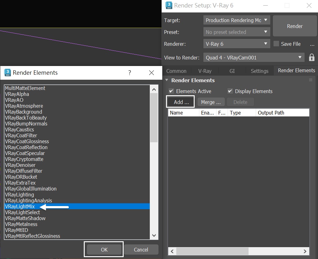
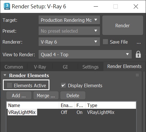
Render Elements
In the Render Setup > Render Elemets tab, add VRayLightMix. This is necessary for relighting the scene in the VFB.
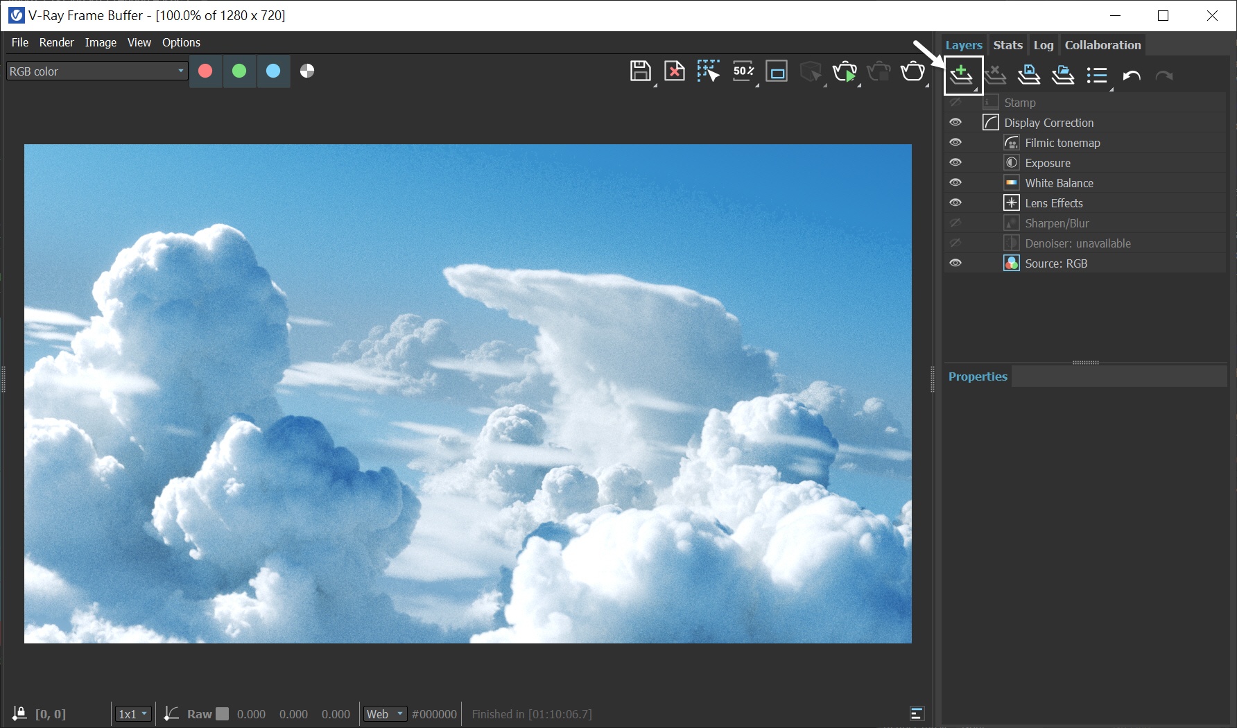
Color Correcting the Daytime Scene with the VFB
Open the V-Ray Frame Buffer and use the Create Layer icon ( ![]() )to add layers for White Balance, Exposure and Filmic Tonemap.
)to add layers for White Balance, Exposure and Filmic Tonemap.
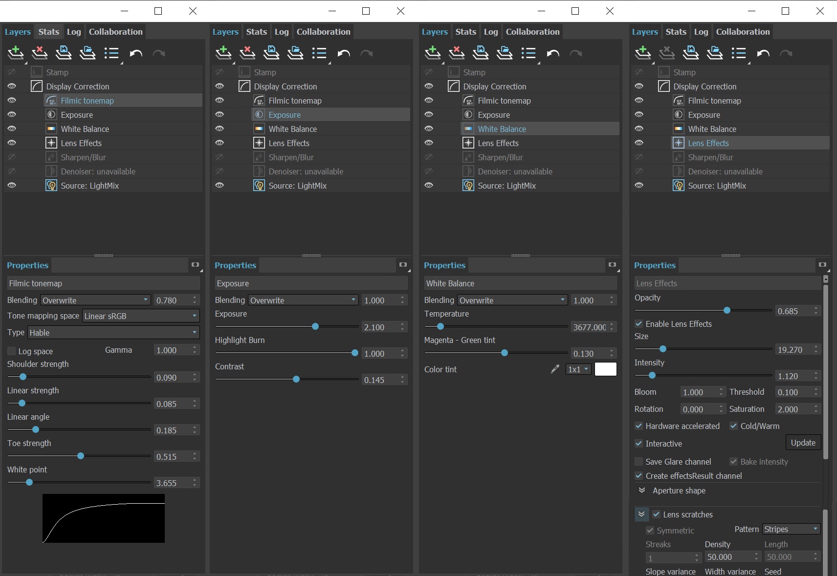
The image is rendered using the V-Ray Frame Buffer. In the current example, the color corrections and post effects are set as follows:
Filmic Tonemap:
- Blending, Override: 0.780
- Type: Hable
- Shoulder strength: 0.090
- Linear strength: 0.085
- Linear angle: 0.185
- Toe strength: 0.515
- White point:3.655
The Filmic Tonemap render element simulates a camera film's response to light, making the scene more realistic.
Exposure:
- Exposure: 2.10
- Highlight Burn: 1.00
- Contrast: 0.145
White Balance:
- Temperature: 3677.0
- Magenta - Green tint: 0.130
Lens Effects:
- Opacity: 0.685
- Size: 19.270
- Intensity: 1.120
- Enable Lens scratches and set its Pattern to Stripes
- Enable Cold/Warm
Feel free to use other values for the post effects, depending on your preferences.
Lighting and Particle effects
Relighting with LightMix
Here we will use LightMix to adjust the ratio between the key light (VRaySun) and the fill-light (VRaySky). We will also decrease the weight of the Environment to make the shot more cinematic.
Set the Source to LightMix.
Change the color swatch of VRaySun001 to orange of RGB(255, 227, 192)
Decrease the weight of the Environment to 0.8. Change the color to RGB(206, 226, 255)
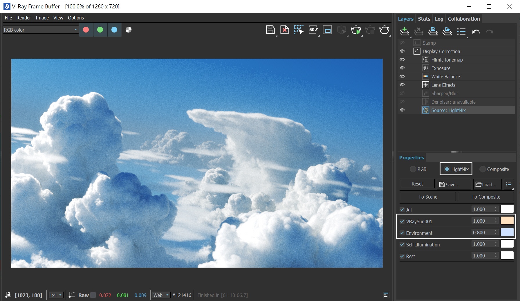
Alternatively, you can load up a render preset from the Daytime_VFB.vfbl file that is provided in the sample scene.

Transfer light changes back to scene
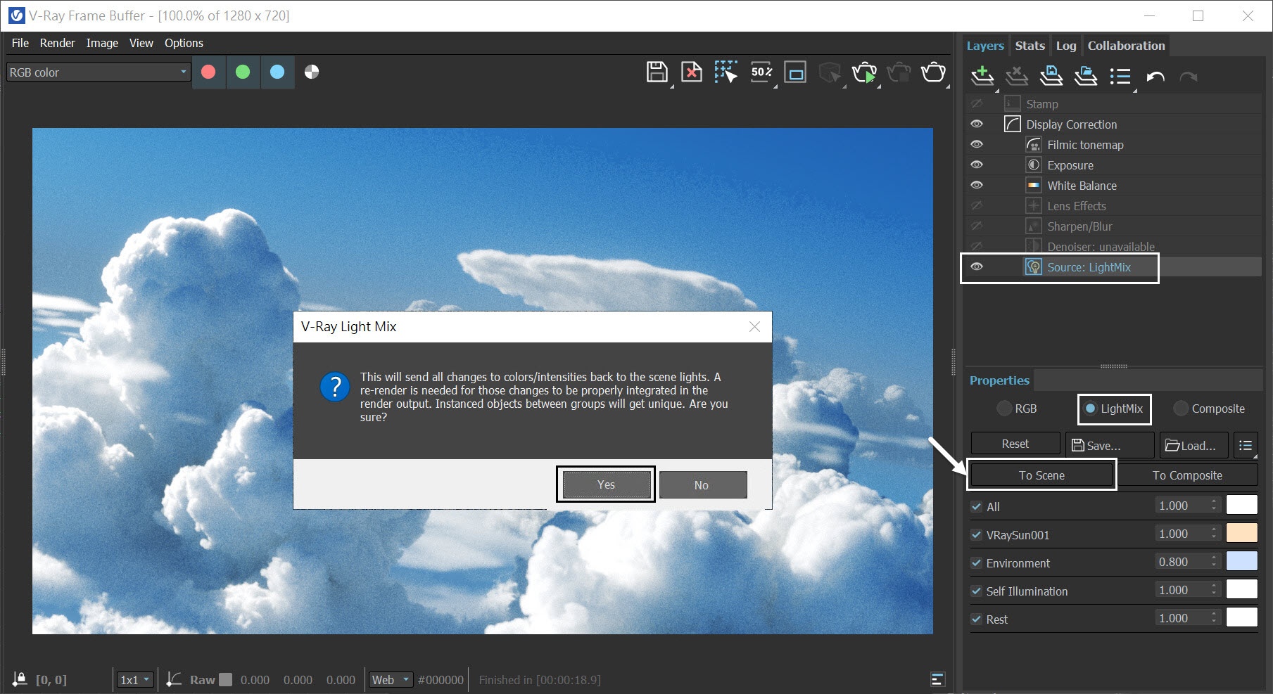
LightMix is a valuable tool that offers precise control over the intensity of individual lights in a scene. This can be particularly useful during look development. However, this feature requires additional sampling during rendering and will slow the render down, when there is already a lot of volumetric data present. The good news is that we can mitigate this issue by using the To Scene button, which allows us to transfer any changes made in LightMix back to the scene without having to repeat the entire render process.
After performing a test render, navigate to the LightMix section in the VFB and click on the To Scene button. This will apply all changes to the colors and intensities of scene items (except for those that were excluded in the previous step).
This prompts a dialogue window, click Yes to confirm.
The To Scene option is only available when the render has stopped. Therefore, it is necessary to perform a quick test render beforehand.
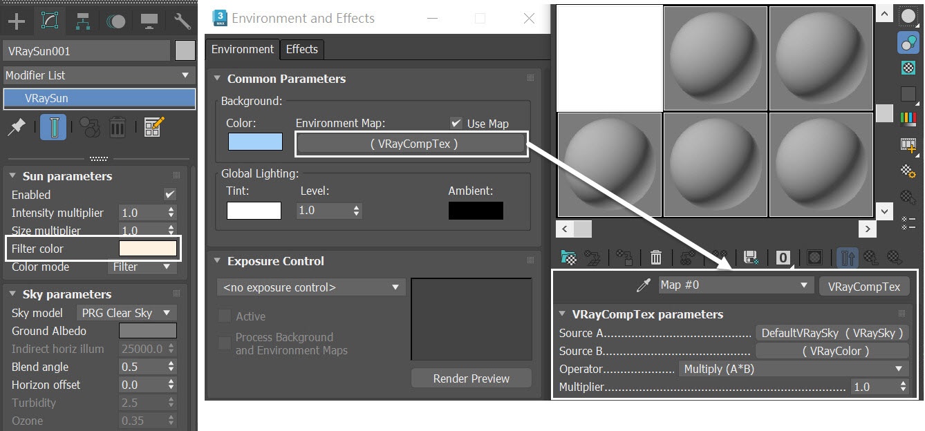
After the transfer, you can check the VRaySun and Environment Map. The VRaySun now has a slightly orange tint, and the VRaySky is multiplied by the VRayColor. Both changes are based on the adjustments we made in LightMix.
Since the light adjustment has now been baked into the scene, let's navigate to VRay > Render Elements and turn off the Element Active option. We are now ready to proceed with the final render for the daytime cloudscape.
And here is the final animation for the daytime cloudscape.
Setup for the Stormy Night Cloudscape
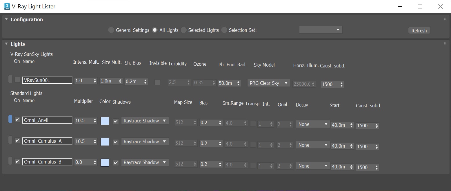
Let's transform the current scene into a stormy night. Take the current state of the daytime scene and save the scene as Cloudscape_stormy.max. First, in the VRay Light Lister, turn off VRaySun and enable the three Omni lights in the scene.
The Multiplier for the Omni_Anvil and Omni_Cumulus_A is controlled by the Noise Controller to create a blinking lightning effect, while the Multiplier for Omni_Cumulus_B has been animated using keyframes.
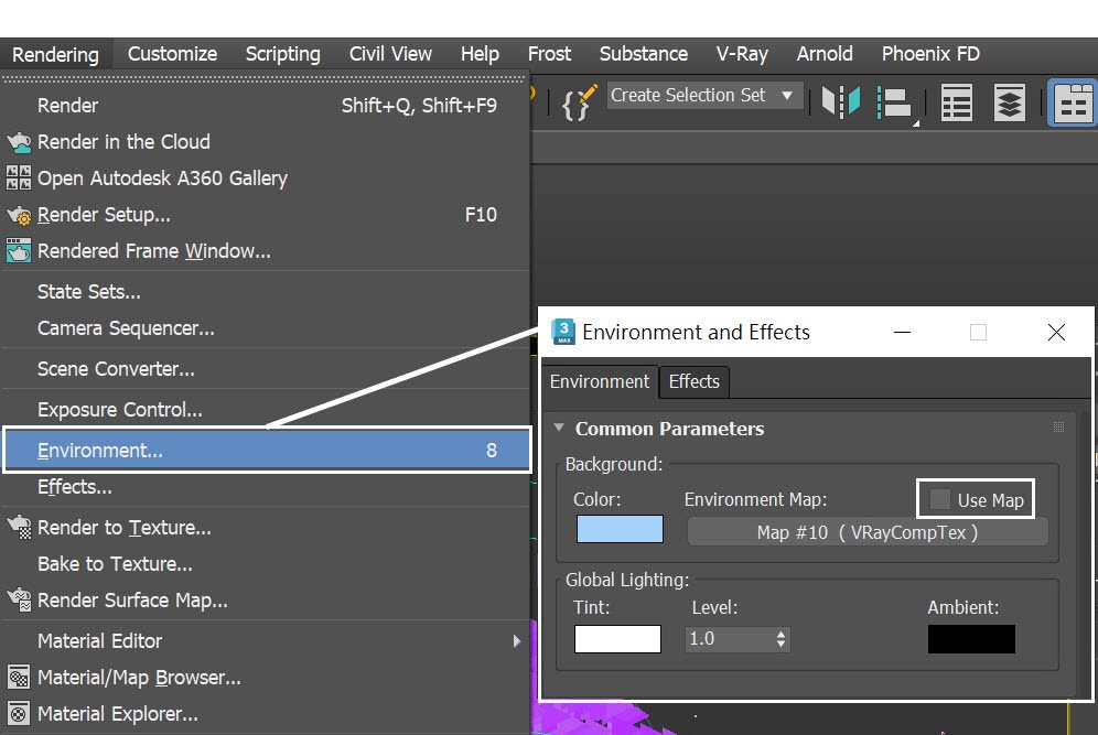
To turn off the VRaySky, navigate to Rendering > Environment > Environment and Effects, and uncheck the Use Map option.
PFlow Setup for the Lightning
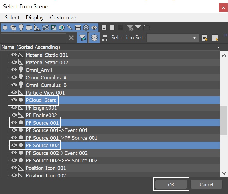
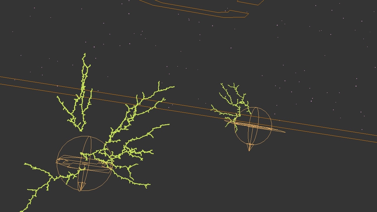
In the Scene Explorer, unhide the PF Source 001, PF Source 002 and PCloud_Stars, to show the PFlow and the stars in the scene.
Here's a preview animation of PFlows and PCloud to give you an idea. In the animation, lightning discharges from the position of Cumulus_A and the Anvil_cloud. You can also see stars in the background.
(Please replace this image with Particles_preview.mp4)
Adjust the VRayVolumeGrid_Fog
Since we want to create a stormy night with high humidity, let's adjust the VRayVolumeGrid_Fog by moving it towards the camera to cover more clouds. Its new position should be XYZ: (1452.0, 11957.0, 0.0).
Next, access the Volumetric Render Settings of the VRayVolumeGrid_Fog. In the Opacity diagram, increase the Y value of the first key point to 0.0003.
Now that we've made the fog thicker, let's optimize render performance by hiding the Chaos_Scatter_Far and VRayVolumeGrid_Cloud_for_scatter_far.
Color Correcting the Nighttime Scene with the VFB
Open the V-Ray Frame Buffer and use the Create Layer icon ( ![]() )to add layers for White Balance, Exposure and Filmic Tonemap.
)to add layers for White Balance, Exposure and Filmic Tonemap.
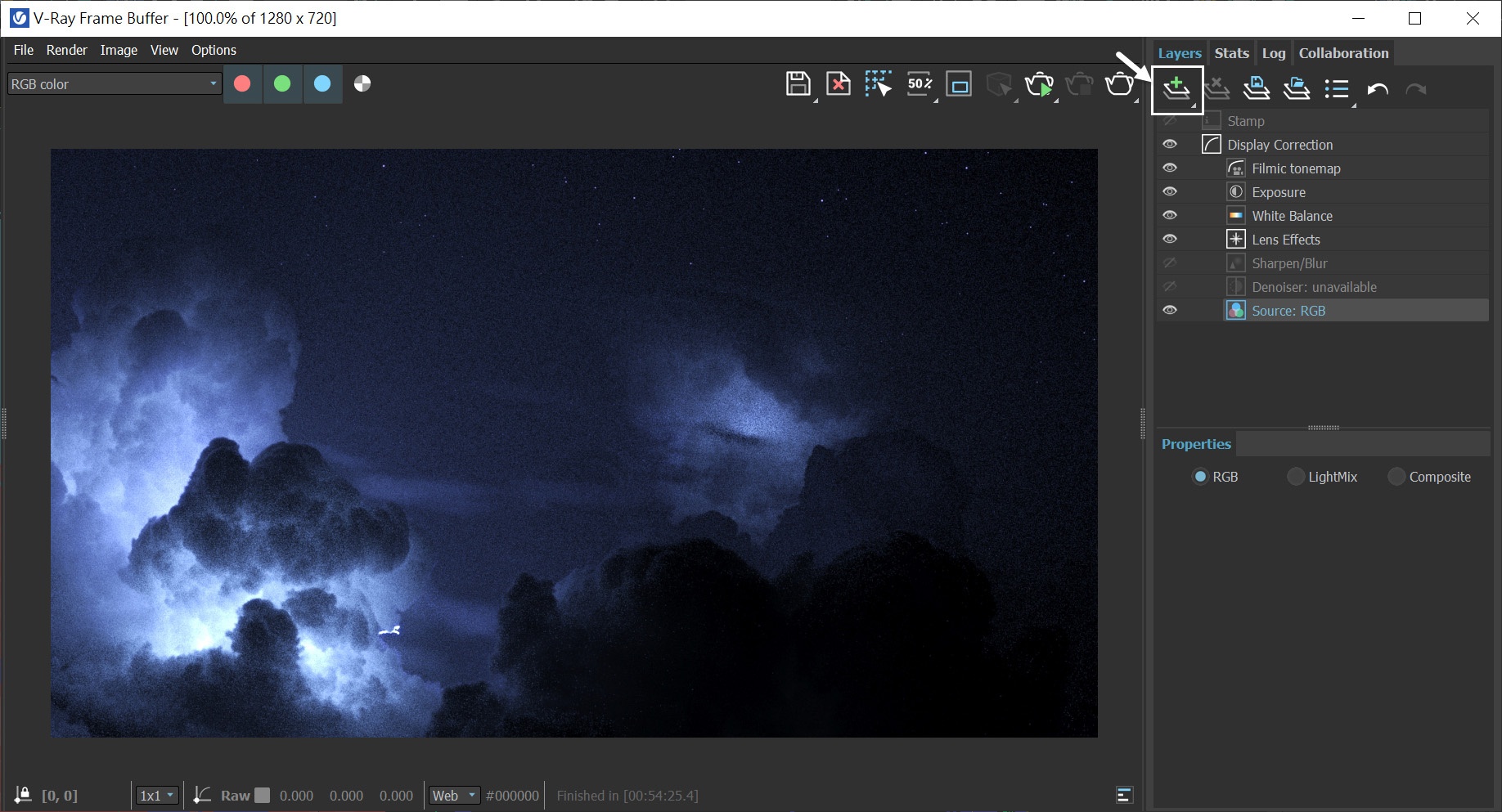
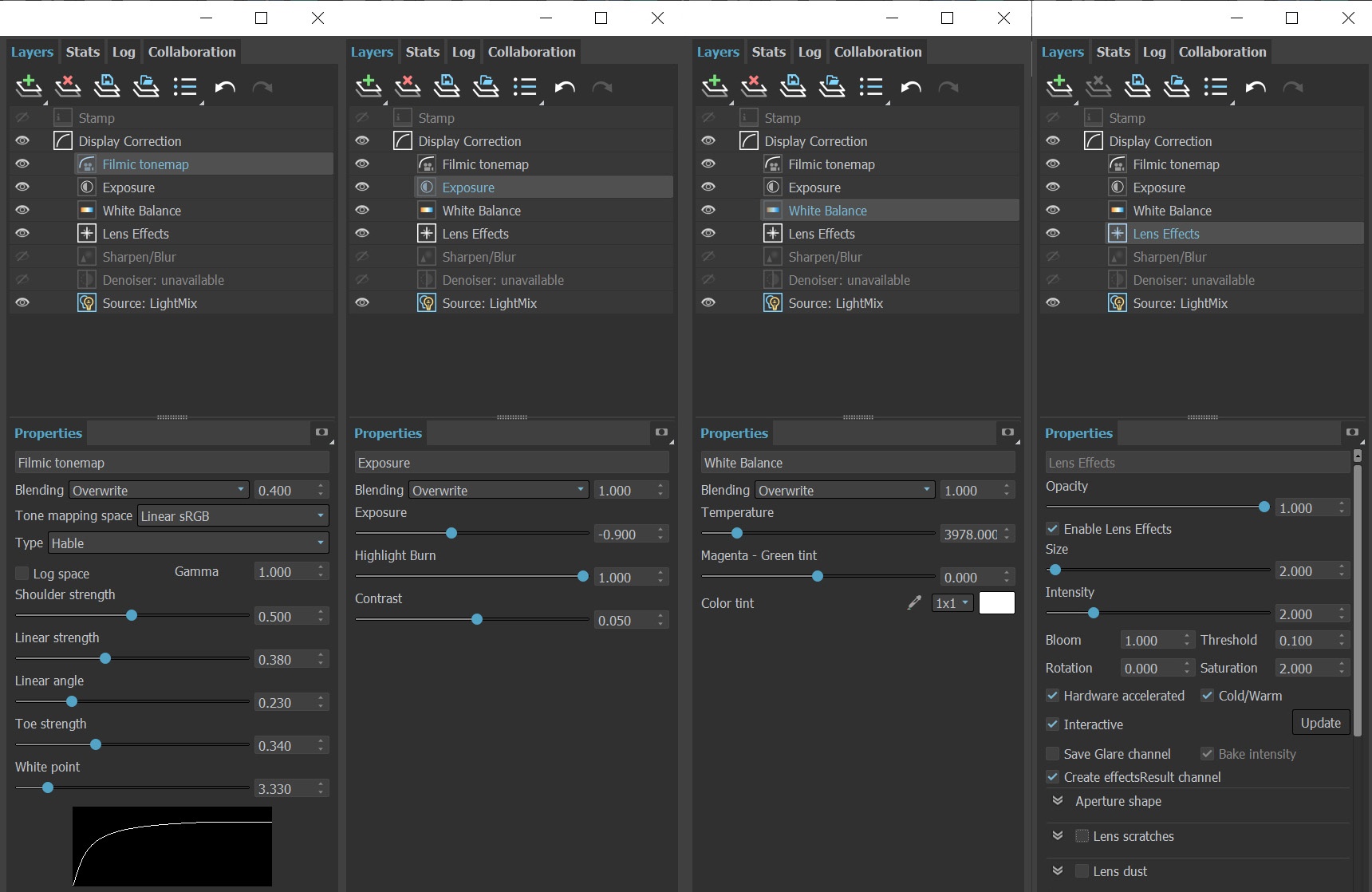
The image is rendered using the V-Ray Frame Buffer. In the current example, the color corrections and post effects are set as follows:
Filmic Tonemap:
- Blending, Override: 0.400
- Type: Hable
- Shoulder strength: 0.500
- Linear strength: 0.380
- Linear angle: 0.230
- Toe strength: 0.340
- White point: 3.330
The Filmic Tonemap render element simulates a camera film's response to light, making the scene more realistic.
Exposure:
- Exposure: -0.90
- Highlight Burn: 1.00
- Contrast: 0.05
White Balance:
- Temperature: 3978.0
- Magenta - Green tint: 0.00
Lens Effects:
- Opacity: 1.000
- Size: 2.000
- Intensity: 2.000
- Enable Cold/Warm
Feel free to use other values for the post effects, depending on your preferences.
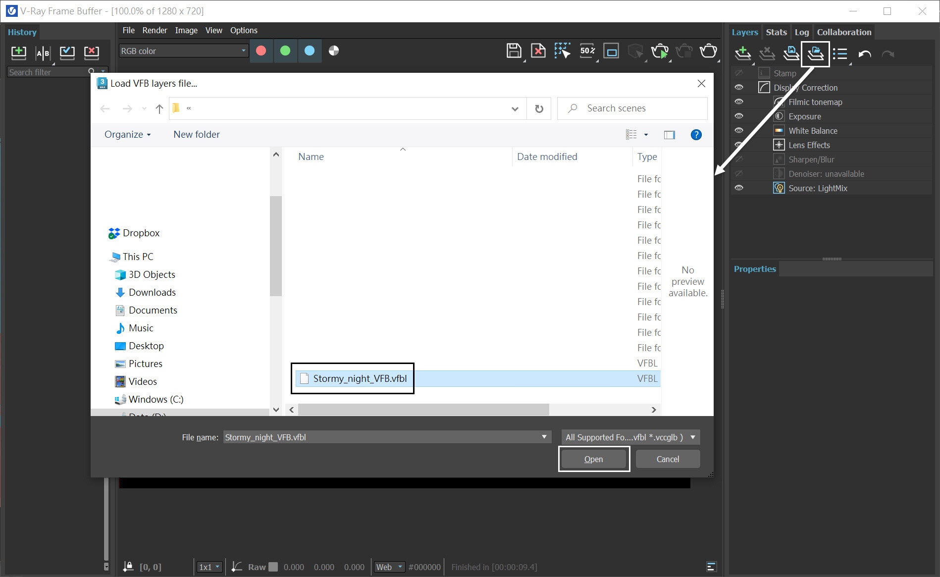
Alternatively, you can load up a render preset from the Stormy_Night_VFB.vfbl file, provided in the sample scene.
And here is the final rendered result for the stormy night cloudscape.
Final composite
We now have sequences of cloudscape scenes for both daytime and nighttime. You can use any compositing software to create an animation that transitions from day to stormy night.
(Please replace this image with Cloudscape_day_and_night.MP4)