![]()
Page History
...
| Section | ||||||||||||||||||
|---|---|---|---|---|---|---|---|---|---|---|---|---|---|---|---|---|---|---|
|

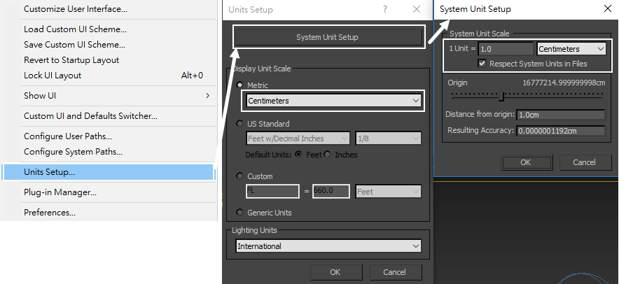
Units Setup
...
| Section | ||||||||||
|---|---|---|---|---|---|---|---|---|---|---|
|
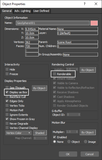
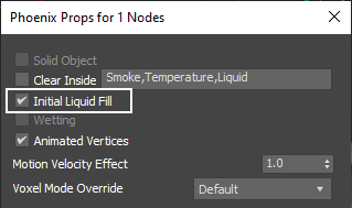
Source Geometry
...
| Section | |||||||||||||||
|---|---|---|---|---|---|---|---|---|---|---|---|---|---|---|---|
|
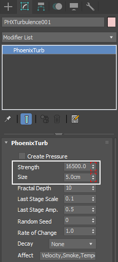
Force
...
| Section | ||||||||||
|---|---|---|---|---|---|---|---|---|---|---|
|
...
Phoenix Simulator
...
Simulation Grid
...
| Section | ||||||||||
|---|---|---|---|---|---|---|---|---|---|---|
| Section | ||||||||||
|
|
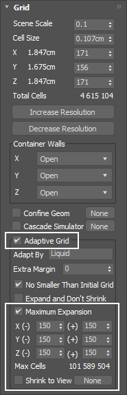
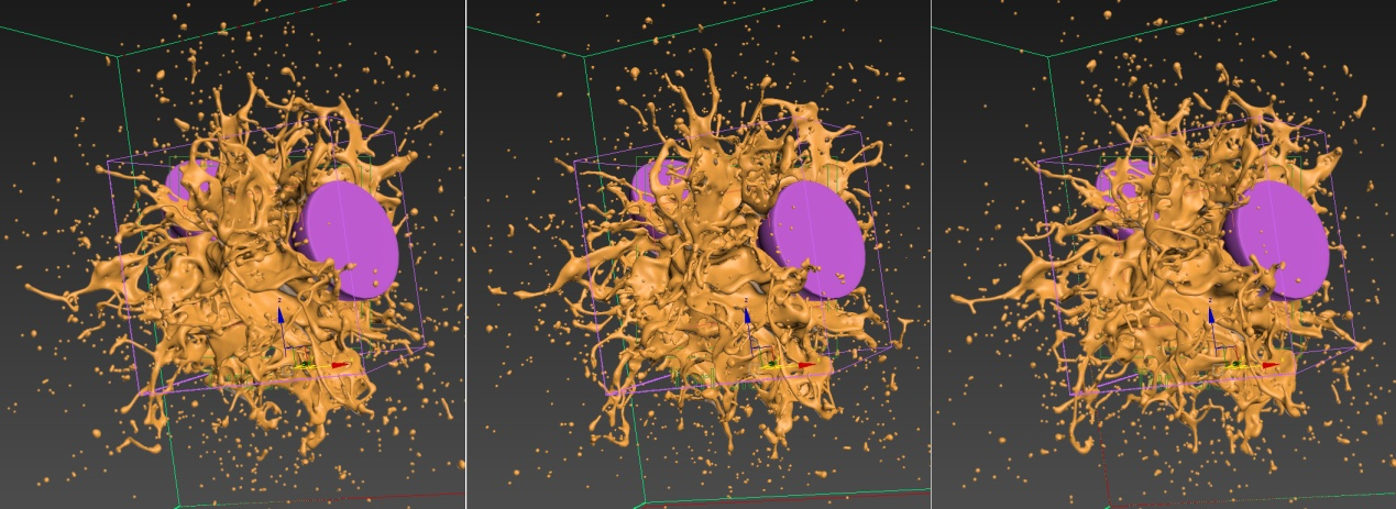
Scene Scale
...
...
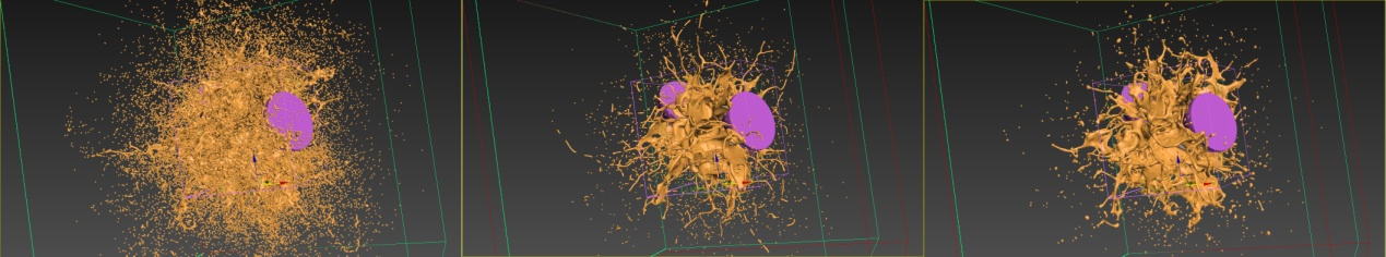
It's time to set the Scene scale.
The image shows three different Scene Scale setups. From left to right those have the following values: 0.1; 0.5; 1.0.
In this
...
specific case there is no big visual difference in the outcome, so pick one of your choice. In this tutorial, we use the value of 0.1.
...
...
...
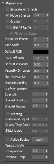
Dynamics
...
| Section | ||||||||||
|---|---|---|---|---|---|---|---|---|---|---|
|
Anchor TimeScale TimeScale
...
 From left to right the Time Scale parameter is set to: 0.7, 0.9, 1.0.
Anchor StepsPerFrame StepsPerFrame
...
 Left image has SPF set to 1 and the right image has SPF set to 2.
Anchor Viscosity Viscosity
...
Left image has Viscosity set to 0 and the right image has a value of 1.
...
| Anchor | ||||
|---|---|---|---|---|
|
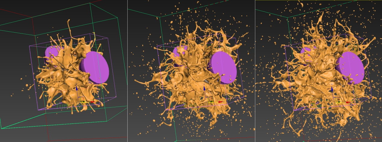
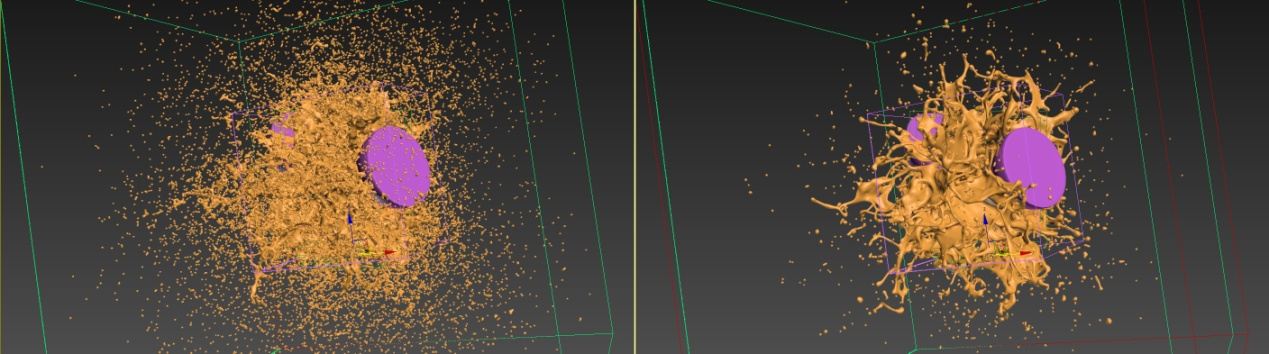
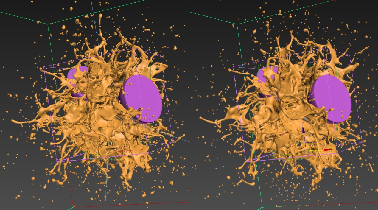
...
Left image: Strength, Droplet Breakup, Droplet Radius are set to 0.0, 0.0 and 2.5. In the middle they have the values of 1.0, 0.0, 2.5. On the right the values are 1.0, 1.0 and 2.5.
...
| Section | ||||||||||
|---|---|---|---|---|---|---|---|---|---|---|
|
Smoothness
...
| Section | ||||||||||
|---|---|---|---|---|---|---|---|---|---|---|
|
| Anchor | ||||
|---|---|---|---|---|
|
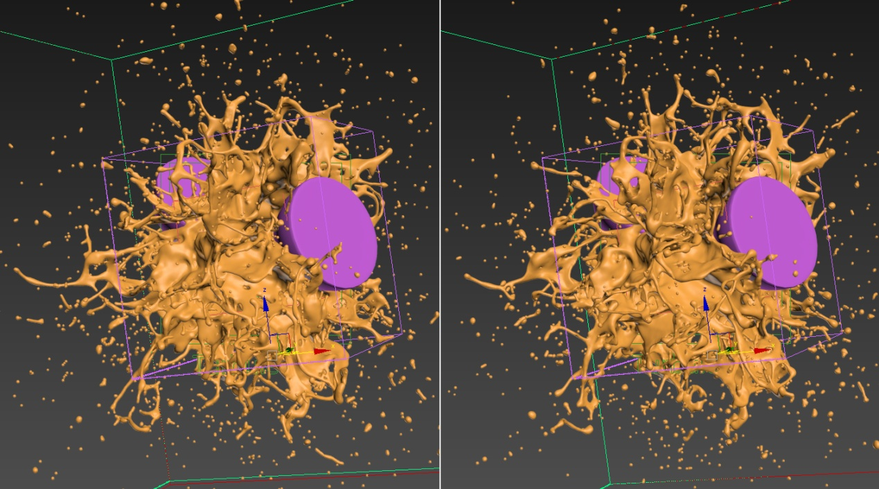
...
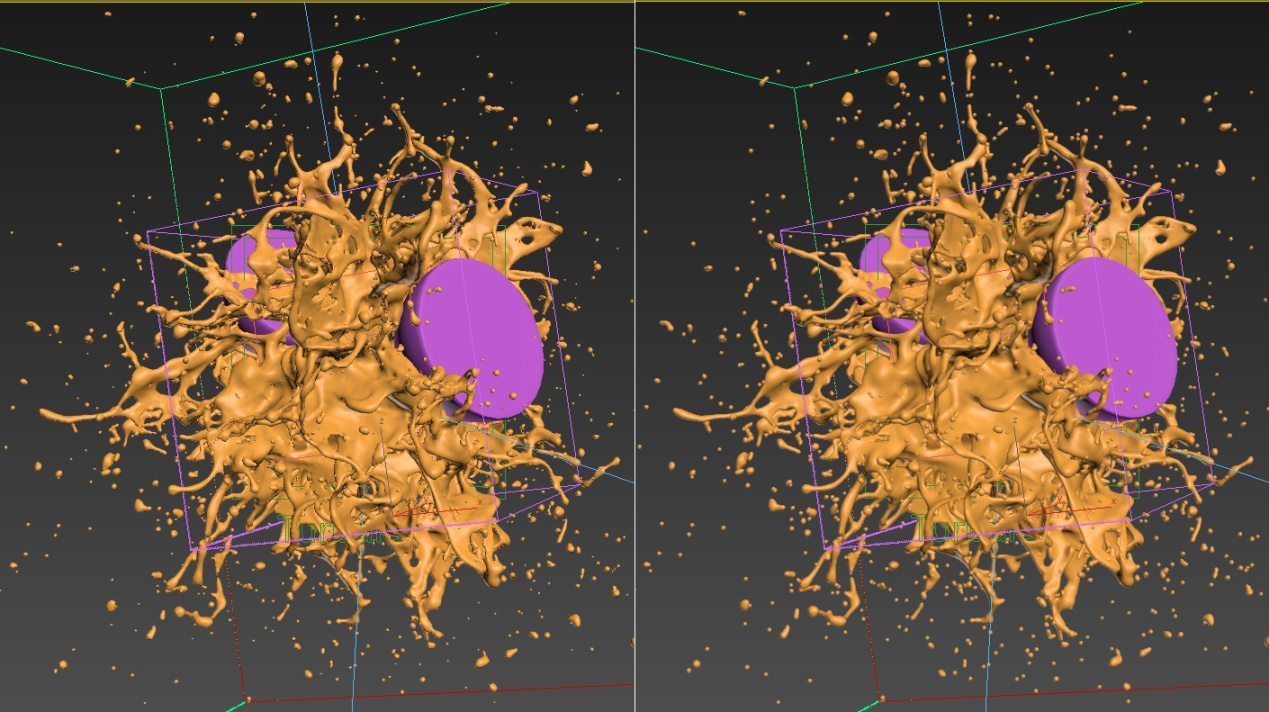 Liquid Particles checkbox is disabled on the left. On the right, the checkbox is enabled.
...
| Section | ||||||||||
|---|---|---|---|---|---|---|---|---|---|---|
|
Lights
...
| Section | ||||||||||
|---|---|---|---|---|---|---|---|---|---|---|
|
...
| Section | ||||||||||
|---|---|---|---|---|---|---|---|---|---|---|
|
...
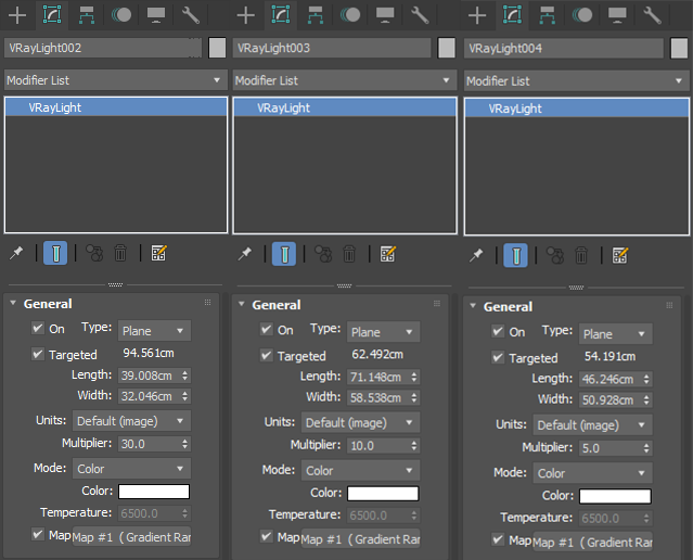
Scene Lights Setup
...
...
|

...
Camera
...
| Section | ||||||||||
|---|---|---|---|---|---|---|---|---|---|---|
|
V-Ray Frame Buffer
...
...
| Section | ||||||||||
|---|---|---|---|---|---|---|---|---|---|---|
|
| UI Text Box | ||
|---|---|---|
| ||
Using V-Ray 5 as our render engine we can take advantage of its Filmic Tonemap in the new VFB. The Filmic tonemap allows you to simulate film response to light with VFB. However, if you are using an older version of V-Ray, you can get a similar effect by using a proper LUT in the VFB. Feel free to use other values for those post effects depending on your preferences. Column | | |
|