This page provides a tutorial on creating a simulation of an exploding orange.
Overview
This is an Intermediate Level tutorial. Even though no previous knowledge of Phoenix is required to follow along, re-purposing the setup shown here to another shot may require a deeper understanding of the host platform's tools, and some modifications of the simulation settings.
Many juice advertisements use the fruit exploding effect in still images and animation. In this tutorial, you will learn how to make this liquid exploding effect with Phoenix.
We will guide you through the fluid simulation itself and show how to use the Phoenix Turbulence force to make the liquid burst out.
We will also show you how different parameters' values (such as Scene Scale, Time Scale, Steps per Frame) give significantly different simulation results, so that you know how to use them in your own simulations.
This simulation requires Phoenix 4.41.02 Nightly Build from 6 Nov 2021 and V-Ray 5 Update 2 for 3ds Max 2018 at least. You can download nightlies from https://nightlies.chaos.com or get the latest official Phoenix and V-Ray from https://download.chaos.com. If you notice a major difference between the results shown here and the behavior of your setup, please reach us using the Support Form.
The Download button below provides you with an archive containing the scene files.

Units Setup
Scale is crucial for the behavior of any simulation. The real-world size of the Simulator in units is important for the simulation dynamics. Large-scale simulations appear to move more slowly, while mid-to-small scale simulations have lots of vigorous movement. When you create your Simulator, you must check the Grid rollout where the real-world extents of the Simulator are shown. If the size of the Simulator in the scene cannot be changed, you can cheat the solver into working as if the scale is larger or smaller by changing the Scene Scale option in the Grid rollout.
The Phoenix solver is not affected by how you choose to view the Display Unit Scale - it is just a matter of convenience.
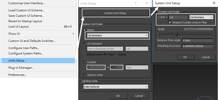
In this scene, we work in centimeters.
Go to Customize → Units Setup and set the Display Unit Scale to Metric Centimeters.
Also, set the System Units such that 1 Unit equals 1 Centimeter.
Source Geometry
Let's start by creating a Geosphere geometry. It will be the only source in the scene for this tutorial. Set its radius to 5.0 cm.
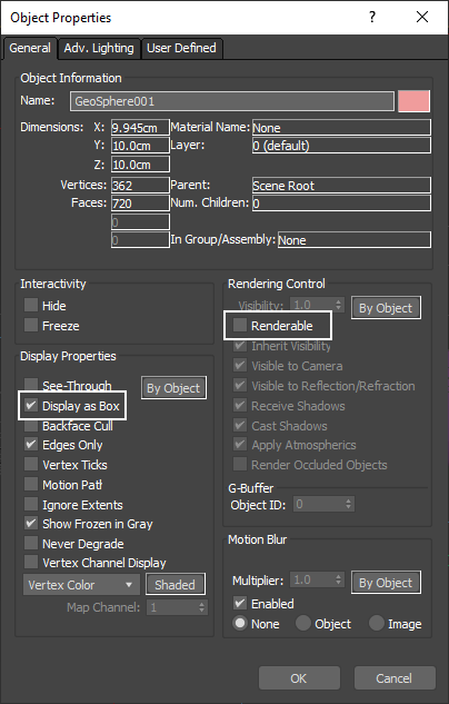
The Geosphere is used only to generate liquid and we don't want it visible in the render view. To achieve that, right-click on the sphere and select Object Properties. Enable Display as Box and disable Renderable options.
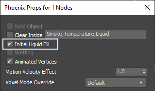
Then, right-click again the sphere and select Phoenix Properties. We want the ball to be filled with liquid at the very beginning of the simulation, so enable the Initial Liquid Fill to secure that.
Force
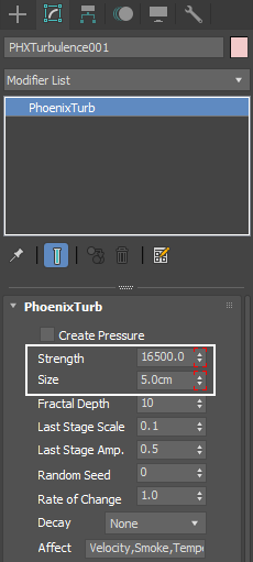
We enter the most critical step of the preparation. Add a Phoenix Turbulence force into the scene. Then, let's set some keyframes to play with the Strength and the Size parameters.
Set the value of Size to 5.0 cm for the first frame. After five frames increase the value to 30 cm. The ultimate goal here is to have the orange juice exploding with lots of detail at the beginning of the simulation, and while the simulation continues, to get less and less of a detail.
Same gradient behavior is desired for the Strength parameter, but in opposite direction. At the beginning of the simulation we expect a quick explosion that won't persist. So, over time decrease the Strength of the turbulence.
From frame 0 to frame 5 increase the Size turbulence from 5 to 30.
From frame 0 to frame 5 decrease the Strength turbulence from 16500 to 0.
Phoenix Simulator
Simulation Grid
Let's move on to creating the simulation grid for the orange juice. Create a Liquid Simulator that encompasses the area around the Geosphere.
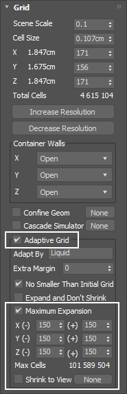
Set the Cell Size to 0.107cm and the X, Y, Z values to 171, 156, 171.
Enable Adaptive Grid. The Adaptive Grid algorithm allows the bounding box of the simulation to dynamically expand on-demand.
Enable Max Expansion: X: (150, 150), Y: (1150, 150), Z: (150, 150) - to save memory and simulation time by limiting the Maximum Size of the simulation grid.
Scene Scale
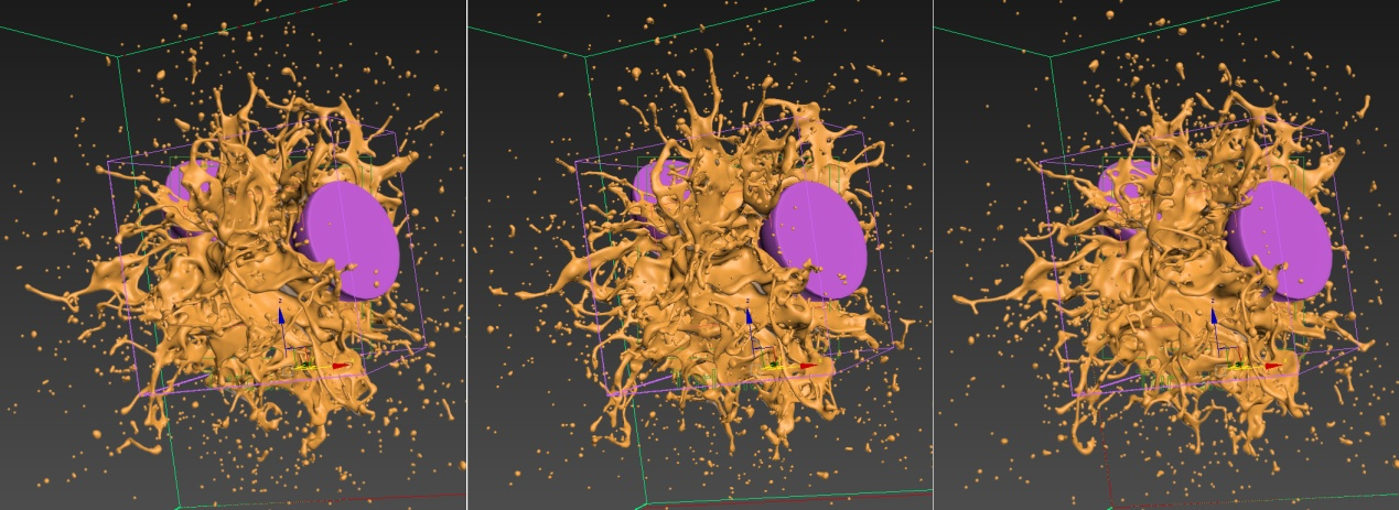
It's time to set the Scene scale.
The image shows three different Scene Scale setups. From left to right those have the following values: 0.1; 0.5; 1.0.
In this specific case there is no big visual difference in the outcome, so pick one of your choice. In this tutorial, we use the value of 0.1.
Dynamics
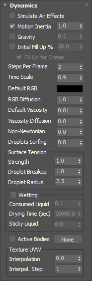
Go to the Dynamics rollout.
Make sure to disable the Gravity option, since we don't want the liquid to actually fall down.
Take a look at the other parameters in this rollout. For ease, here are the set values:
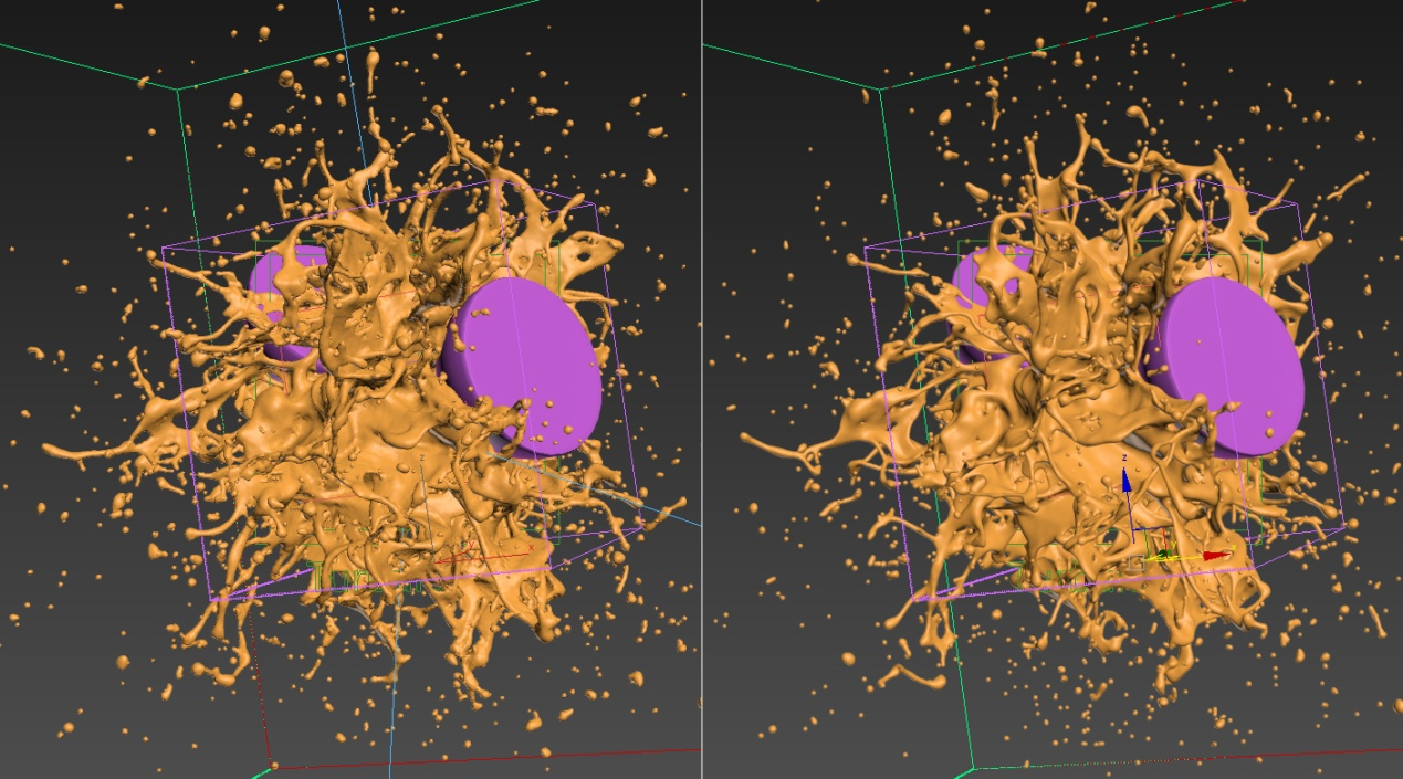
Steps Per Frame is set to 2. In the comparison example you can see how dramatic SPF is affecting the liquid mesh. The default value of 1 makes the liquid too diffused. Check a comparison image for the Steps Per Frame parameter.
Time Scale is set to 0.9. Note that, the lower the Time Scale, the slower the movement of the liquid will be. It also affects the so called "sticky look". Check the comparison Time scale example below.
Default Viscosity is set to 0.01. Check the comparison example of Viscosity below.
Surface Tension Strength controls the force produced by the curvature of the liquid surface. This parameter plays an important role in small-scale liquid simulations because an accurate simulation of surface tension indicates the small scale to the audience. Lower Surface Tension values will cause the liquid to easily break apart into individual liquid particles, while higher values will make it harder for the liquid surface to split and will hold the liquid particles together. With high Surface Tension, when an external force affects the liquid, it would either stretch out into tendrils, or split into large droplets.
Droplet Breakup controls the balance between tendrils or droplets formed by the liquid.
Droplet Radius controls the radius of the droplets formed by the Droplet Breakup parameter.
Check the result of experimenting with those Surface Tension parameters below. In this tutorial we use the balanced values of 1.0 for Droplet Breakup and Strength, and 2.5 for Droplet Radius.
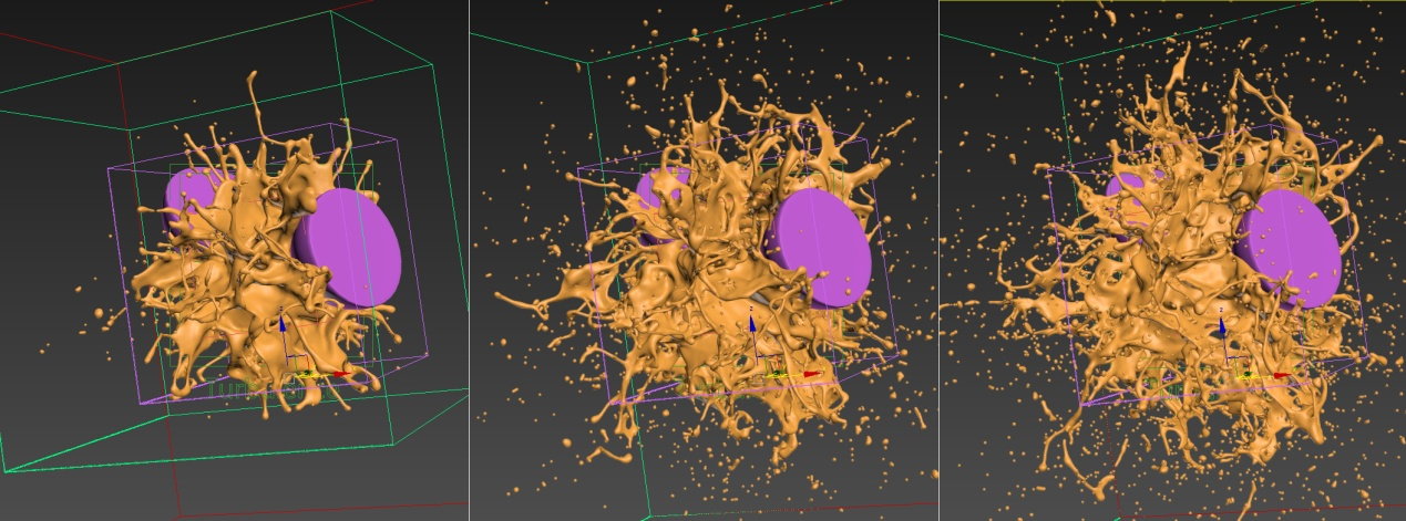 From left to right the Time Scale parameter is set to: 0.7, 0.9, 1.0.
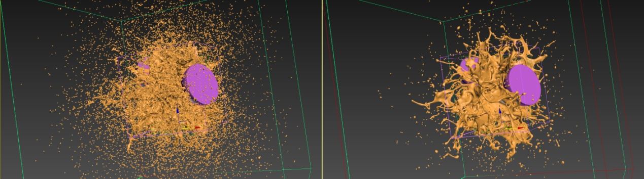 Left image has SPF set to 1 and the right image has SPF set to 2.
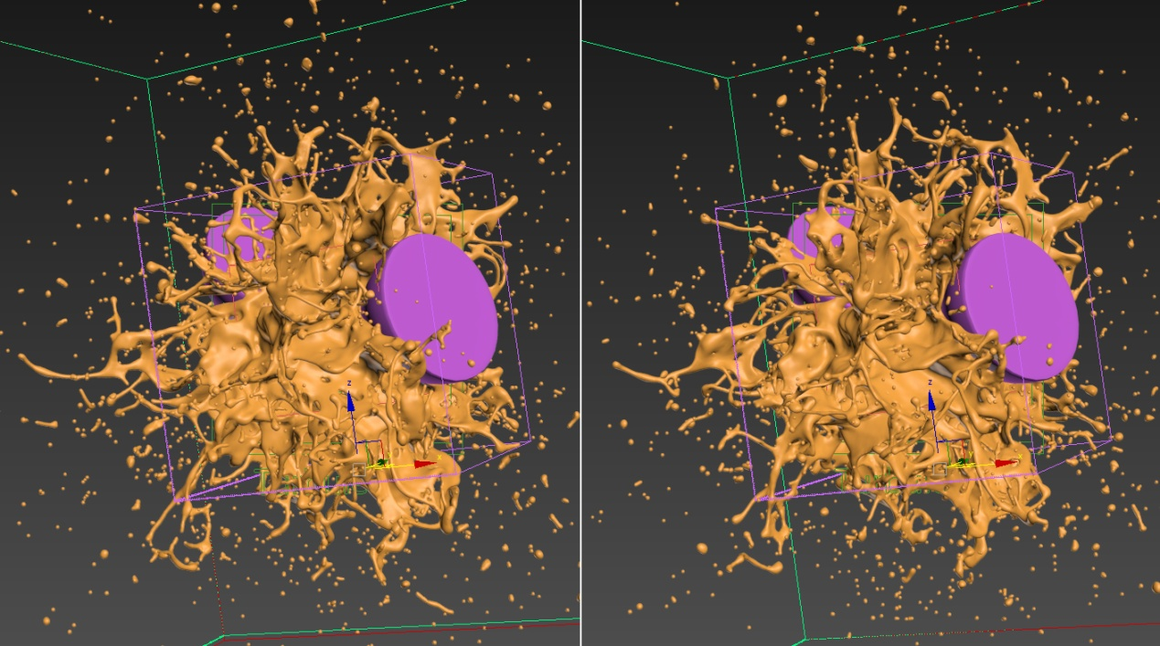
Left image has Viscosity set to 0 and the right image has a value of 1.
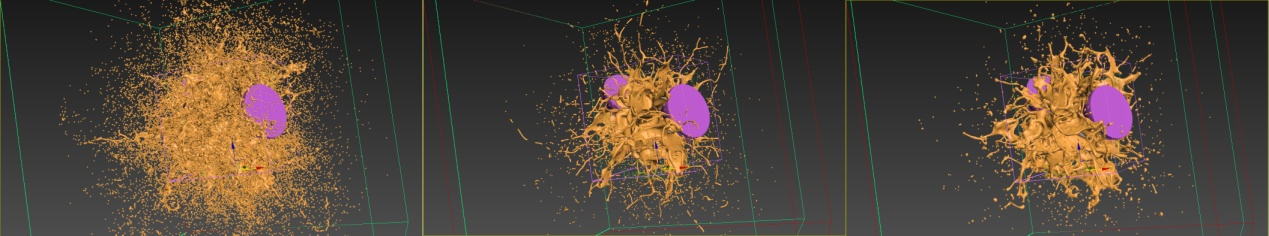
Left image: Strength, Droplet Breakup, Droplet Radius are set to 0.0, 0.0 and 2.5. In the middle they have the values of 1.0, 0.0, 2.5. On the right the values are 1.0, 1.0 and 2.5.
Output
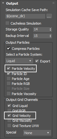
Open the Output rollout.
Make sure to enable the Velocity option from the Output Grid Channels panel. It is useful if you want to use Motion Blur during rendering.
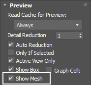
Preview
Go to the Preview rollout and enable the Show Mesh option. This will display the liquid mesh directly in the viewport.
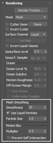
Rendering
In the Rendering rollout we lower the Motion Blur's Multiplier in order to make the final effect more subtle.
Enable the Use Liquid Particles option. This method overcomes the limitations of the basic smoothing without particles, which can flicker in animation and cause small formations in the mesh to shrink. Check the example below showing how the simulation looks with and without this option enabled. There is a very subtle difference.
Smoothness
Let's take a look at how the Smoothness parameter affects the whole simulation.
On the left, you see a simulation with Smoothness set to 0. On the right-hand side Smoothness is increased to 20.
Notice how a value of 20 can significantly reduce the banding that is usually seen in grid simulations. The higher the Smoothness value, the smoother the result, but the mesh will require more time to calculate.
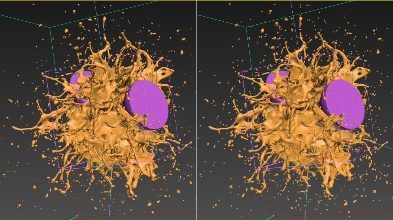 Liquid Particles checkbox is disabled on the left. On the right, the checkbox is enabled.
Orange Juice Material
In order to get a realistic looking orange juice, you generally will need to go through a lot of testing and fine adjustments of the material.
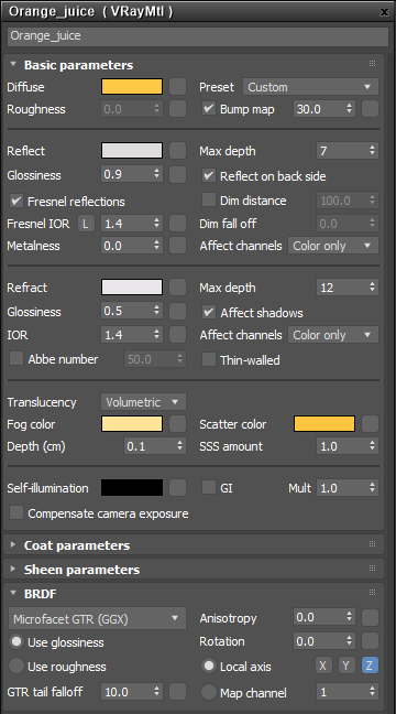
But we have you backed up! In this tutorial we use a VRayMtl with the settings from the image.
Feel free to experiment until you find the best fit for your orange juice. But be aware that the right lighting plays a vital role in a good-looking render.
Diffuse color - R: 250 G: 149 B: 15;
Reflection color - R: 188 G: 184 B: 186;
Reflection Glossiness is set to 0.9;
Fresnel IOR is set to 1.4;
Refraction color - R: 207 G: 203 B: 209;
Refraction Glossiness is set to 0.5;
IOR is set to 1.4;
Translucency - Volumetric;
Fog color - R: 254 G: 199 B: 80;
Depth is set to 0.1 cm;
Scatter color - R: 254 G: 144 B: 12.
Lights
We move on to adding Lights to our scene.
There is a V-Ray Dome light set as an environment light. Aside from it, there are three V-Ray Plane Lights - one on top, one on the side, and one at the bottom.
The size and intensity of each light are shown here.
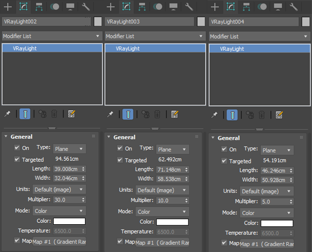
Each light is using a GradientRamp as a mask, so that the light will be softer and looking natural.
Set the Mapping to Explicit Map Channel.
Set the Blur to 4.0.
Set the Gradient Type to Box.
In the Output tab, enable Invert.

Camera
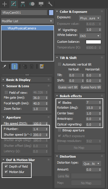
Here is a suggestion of how to set up a Physical Camera for this scene.
The Focus Distance is set to 81.208.
Aperture → F-Number is set to 1.4.
Aperture → Shutter Speed is set to 200.0.
Color & Exposure → White Balance is set to D65.
Enable both the Depth of field and Motion blur.
In the Bokeh effects tab, the Blades option is enabled and set to 7, with a Rotation of 15. Center bias is set to 1.0.
Feel free to adjust those parameters in a way they work best for you.
V-Ray Frame Buffer
The final image is rendered using the V-Ray Frame Buffer with the color corrections and post effects set to:
Filmic Tonemap
- Type - Power Curve;
- Toe length: 0.178;
- Toe strength: 0.274;
- Contrast: 0.706;
- Shoulder length: 0.508;
- Shoulder strength: 0.355;
- White point: 3.330
Hue / Saturation
- Hue: 4.00;
- Saturation: - 0.040;
Sharpen/Blur
- Sharpen amount: 3;
- Sharpen radius: 1;
- Blur radius: 1;
Feel free to use other values for those post effects depending on your preferences.
Using V-Ray 5 as our render engine we can take advantage of its Filmic Tonemap in the new VFB. The Filmic tonemap allows you to simulate film response to light with VFB. However, if you are using an older version of V-Ray, you can get a similar effect by using a proper LUT in the VFB.