This page provides a tutorial on creating a Milk and Chocolate fusion simulation in 3ds Max.
Overview
This is an Intermediate Level tutorial. Even though no previous knowledge of Phoenix is required to follow along, re-purposing the setup shown here to another shot may require a deeper understanding of the host platform's tools, and some modifications of the simulation settings.
Requires Phoenix 3.11.01 Nightly Build ID 28305 and V-Ray 3.60.04 Official Release for 3ds Max 2015 or newer. You can download nightlies from https://nightlies.chaos.com or get the latest official Phoenix and V-Ray from https://download.chaos.com. If you notice a major difference between the results shown here and the behavior of your setup, please reach us using the Support Form.
In this tutorial, we guide you through the creation of a fusion effect resulting from the splash of two fluids - milk and chocolate. For this goal, we create two liquid emitters, one for each liquid type. By using a Blend Material, we set the appearance of the mixture.
The two liquids are simulated with different RGB each, and then the grid RGB channel is extracted via a Phoenix Grid Texture and used as a mask for the Blend Material. We use Surface Tension to keep the liquid particles packed together in a smooth mesh and only allow them to break up into larger droplets.
To make the liquid mesh look even smoother, as a real milky-looking liquid, we use the Phoenix smoothing tools found in the Input and Rendering rollouts of the Simulator.
The Download button below provides you with an archive containing the start and end scenes as a reference.
System Units
Scale is crucial for the behavior of any simulation. The real-world size of the Simulator in units is important for the simulation dynamics. Large-scale simulations appear to move more slowly, while mid-to-small scale simulations have lots of vigorous movement. When you create your Simulator, you must check the Grid rollout where the real-world extents of the Simulator are shown. If the size of the Simulator in the scene cannot be changed, you can cheat the solver into working as if the scale is larger or smaller by changing the Scene Scale option in the Grid rollout.
The Phoenix solver is not affected by how you choose to view the Display Unit Scale - it is just a matter of convenience.
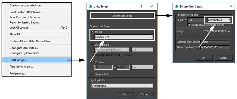
Go to Customize → Units Setup and set Display Unit Scale to Metric Centimeters.
Also, set the System Units such that 1 Unit equals 1 Centimeter.
Scene Setup
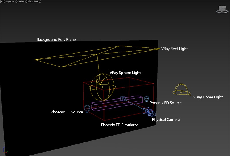
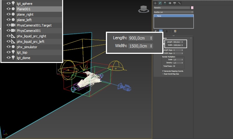
For a better understanding of how the scene components work together, take a look at the Scene Setup image. This is how the finished scene will be laid out.
The two liquid emitters are positioned facing each other, with the Chocolate emitter on the left and the Milk emitter on the right.
Three lights are used in the scene:
A V-Ray Dome Light provides an overall diffuse illumination.
A V-Ray Rect Light is placed above the Phoenix Simulator and acts as the key.
A V-Ray Sphere Light provides backlighting for translucency.
A dark poly plane is positioned behind the Phoenix Simulator to serve as a background.
Simulation Setup
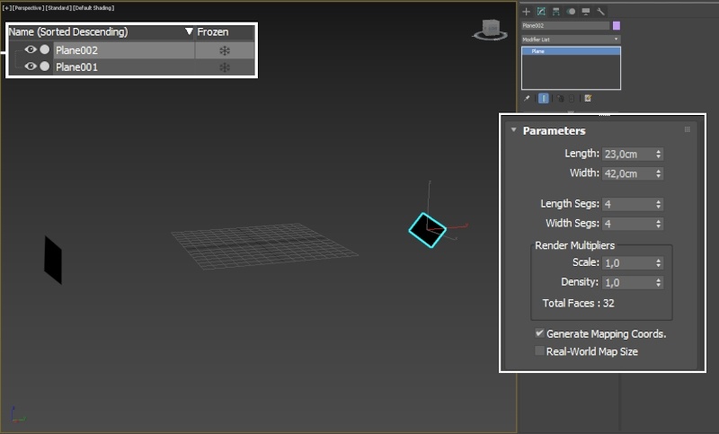
The liquid emitter geometries used in this tutorial are two 3ds Max Primitive Planes.
If you'd like your setup to be identical to the provided scene files, here are the exact sizes and transformations of the planes:
- Left plane:
Length/Width: 23/42cm;
Translate: [0, -185, 0];
Rotate: [57, -148, -3.5].
- Right plane:
Length/Width: 23/42cm;
Translate: [0, 185, 0];
Rotate: [-124.5 , 11 , 0].
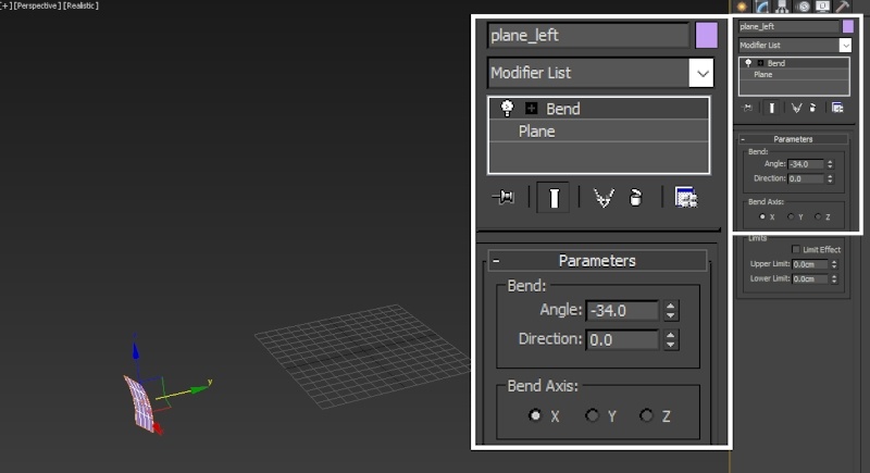
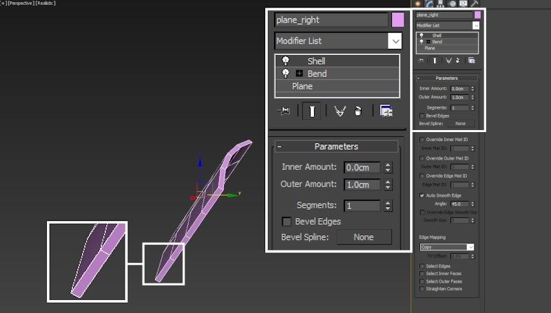
Add a Bend modifier to give the planes a slight curve. This will spread the emitted fluid in an arc rather than producing a cubic shape.
Change the Bend Axis for both planes to X.
If you'd like your setup to be identical to the provided scene files, here are the Bend Angle values for the planes:
Left Plane: [Bend Angle: -34]
Right Plane: [Bend Angle: -25]
You may want to experiment with the Bend Angle parameter - different values will produce slightly different results.
Add a Shell modifier to both planes and leave its settings at their default values.
The Shell modifier is applied to give the geometries thickness. This allows Phoenix to properly calculate the volume of the object that you're using for the emission.
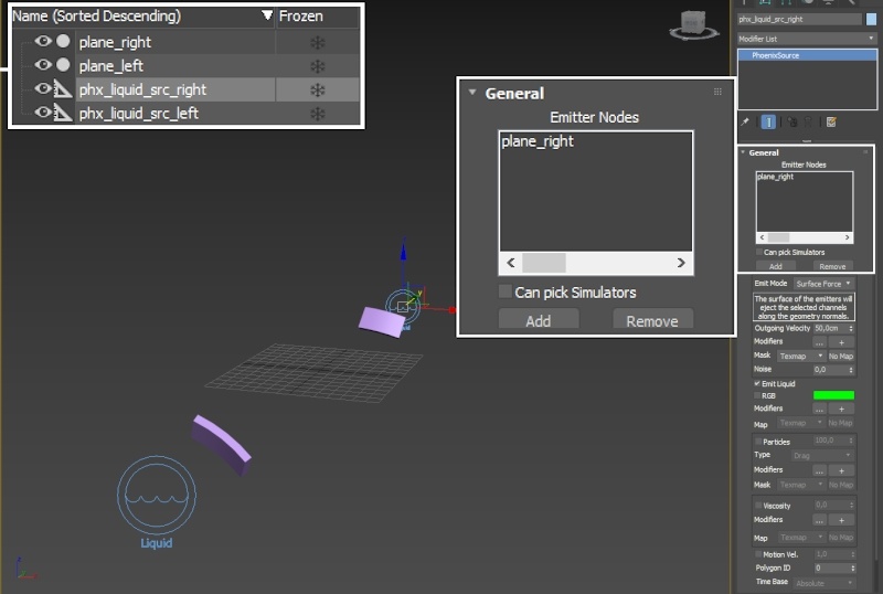
Create two Phoenix Liquid Sources. Position them next to the planes and give them meaningful names so you can keep organized and focused.
Select the Phoenix Source on the right and use the Add button to add the poly plane on the right as its source geometry.
Repeat this step for the Phoenix Source on the left.
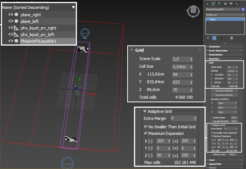
Create a Phoenix Liquid Simulator that envelops both source geometry objects.
Under the Grid rollout, set the Scene Scale to 2. The Scene Scale parameter will affect most of the dynamics in the Simulator. A smaller value will produce splashier, more turbulent movement while a larger Scene Scale will give the impression of a heavier, more inert fluid. You may experiment with this parameter but keep in mind that you will also have to adjust the Outgoing Velocity of the Phoenix Sources as well.
Enable Adaptive Grid and Maximum Expansion. The red box in the screenshot to the right is a preview of the Maximum Bounds for the simulation. Adaptive Grid is a huge time saver - the initial grid is dynamically expanded to accommodate the movement of the fluids, cutting down on both processing time and memory. If you notice any clipping, increase the Extra Margin to a value of 5 - 10. This will add a few extra voxels at the borders during adaptation.
If you'd like your setup to be identical to the provided scene file, here are the exact values for the Grid parameters:
Cell Size is set to 0.64cm for the final simulation.
The X/Y/Z dimensions of the Grid are 90/650/70 respectively.
The Adaptive Grid Maximum Expansion settings are [200, 200] for X, [0, 0] for Y and [50, 200] for Z.
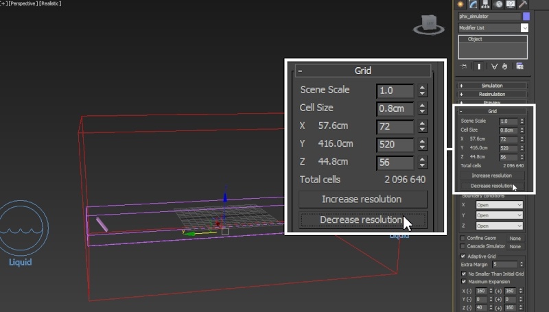
Now that we have a Simulator, Sources and source geometry, we are ready to start the R&D process.
Reduce the resolution of the grid by hitting the Decrease Resolution button once. This will reduce the number of voxels in the grid by half, thus reducing the simulation time.
You can easily go back to the final resolution by pressing the Increase Resolution button.
Hit the Start button and wait for 50 or so frames.
To get a preview of the liquid surface, you can enable Preview → Show Mesh.
Here's how the simulation looks so far:
You can see from the Preview Animation above that the default behavior of the Phoenix Liquid Source is to emit liquid from the surface of the source geometry. Phoenix provides you with 2 ways to direct the discharge:
- Using Polygon/Face IDs to limit the emission to manually specified faces.
- Using Discharge Modifiers on the Liquid Source to limit the emission based on the position, orientation or animation speed of the faces.
In this tutorial, we use the simpler option 1.
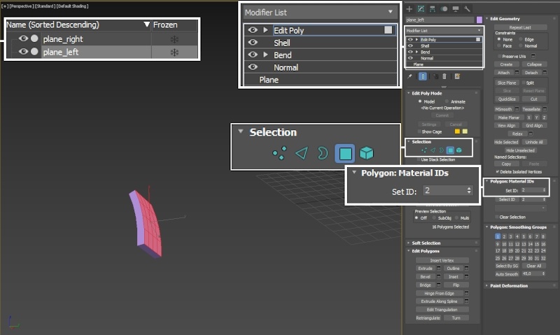
Add an Edit Poly modifier and go into Face selection mode. Select the faces pointing towards the Origin and give them a unique Material ID. By default, all faces have an ID of 1, so switching the ID to 2 for the selected faces should do the job.
The Phoenix Liquid Source in 3ds Max can use the polygon face IDs as a 'mask' - only the faces with a given ID will be used for emission.
Repeat this step for the other poly plane.
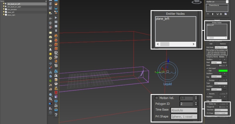
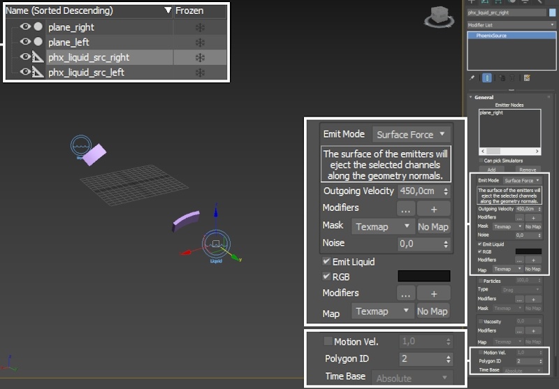
Select each Phoenix Liquid Source and set the Polygon ID parameter to the same value that you gave the source geometry faces in the previous step.
This will force the liquid source to only emit from the polygons with the specified ID value.
No Polygon IDs for the Liquid Source
With Polygon IDs for the Liquid Source
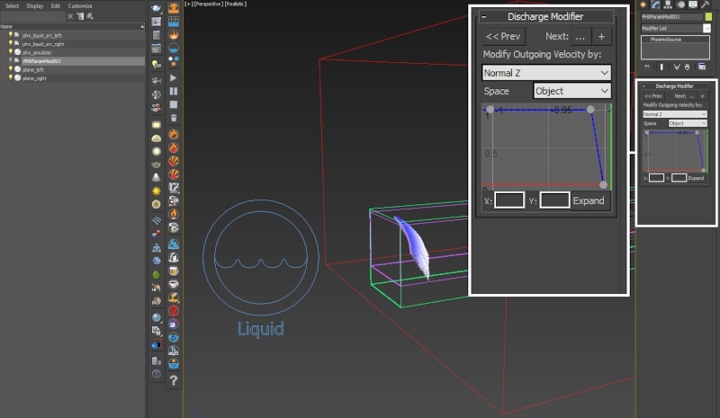
Discharge Modifiers allow for advanced control which you might need for more complex simulations. If you'd like to use Discharge Modifiers instead of Polygon IDs with this setup, click the + icon under the Outgoing Velocity parameter of the Liquid Source.
Set the Modify Outgoing Velocity by option to Normal Z and the Space to Object.
When the Space parameter is set to Object, the normals of the geometry are computed before any transformation (such as moving or rotating) are applied. Because the source geometry was created flat on the XY axis and then moved and rotated into position, the faces pointing towards the origin actually have their object space normals pointing in either negative or positive Z.
Please refer to the Discharge Modifiers documentation page which contains a lot of information, example settings, and pictures.
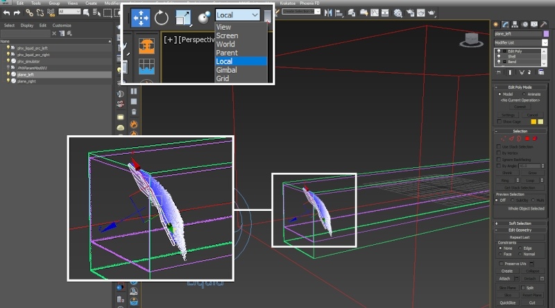
An easy way to check the Object Space orientation of your geometry would be to select it, invoke the Move tool and set the space to Local. The arrows of the move tool's gizmo will show you the object space orientation of your geometry.
In this example you can see that the blue arrow (Z axis) is pointing away from the origin. Therefore, if you want the emission to go towards the origin, you need to setup the Discharge modifier such that the points on the graph are as follows:
Left point: X: -1 , Y: 1
Right point: X: -0.9, Y: 1
The X-values correspond to the direction of the normal (-1 being the opposite of the blue arrow, and 1 being exactly along it), and the Y-values correspond to the resulting discharge multiplier.
This setup on the picture above is saying the following: "If the normal of the face is pointing in -Z in local space, emit with a discharge multiplier of 1. Otherwise, set the multiplier to 0."
Currently, the emission is too weak. Instead of colliding with each other and producing an interesting splash, the liquids emitted from the two sources simply fall down.
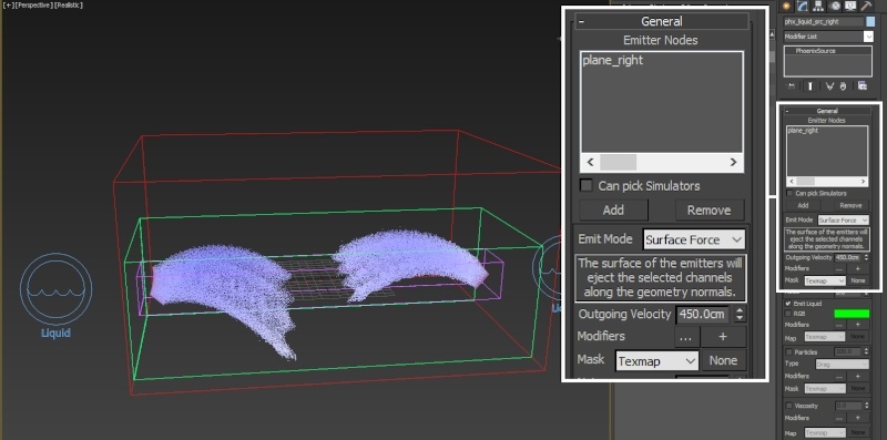
Increase the Outgoing Velocity parameter of the Liquid Sources. If you'd like your setup to be identical to the provided scene files, here are the exact values:
Left Phoenix Source: [Outgoing Velocity: 400cm].
Right Phoenix Source: [Outgoing Velocity: 450cm].
Here is the simulation with a higher Outgoing Velocity rate:
Note the stepping in the emission. This is caused by a combination of factors - the high Outgoing Velocity of the source and the low Steps Per Frame of the Simulator.
The Steps Per Frame (SPF) parameter controls how many calculations are made between two consecutive frames. This includes the emitters as well. If you see stepping in the emission, increasing the SPF is most likely your best bet.
Increasing the SPF to a very high value may seem like a good idea - after all, this will give you a perfectly smooth emission, so why not?
The Steps Per Frame parameter affects the simulation time significantly - each step is calculated separately so increasing the SPF twice will also increase the simulation time twice. You should only go as high as needed, and not more.
Furthermore, the higher the SPF is, the less detailed your simulation becomes. The reason behind this is that each step is calculated by scaling the velocities in your simulation, moving the liquid, and repeating. This tends to 'smooth-out' chaotic motion which is usually a requirement for turbulent, splashy or explosive effects.
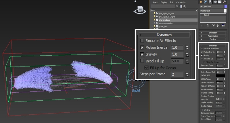
Select the Phoenix Liquid Simulator and set the Steps Per Frame parameter to 2. This value should suffice for the current setup.
Steps Per Frame: 2
Steps Per Frame: 4
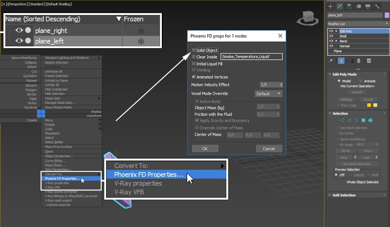
Select both poly planes, Right-Mouse-Button click → Chaos Phoenix Properties...
Disable the Solid Object option under the properties window.
When the source geometry is solid and emitting in Surface mode, the velocity field calculation takes said geometry into account and it acts as an obstacle.
If you disable the Solid Object option, the fluid will not (indirectly, through the influence of the velocity field) interact with the source geometry at all.
Because the liquid is moving too fast, we will reduce the Gravity and Time Scale from the Dynamics rollout of the Simulator.
Set the Gravity to 0.5. The Gravity parameter is self-explanatory - the liquid will fall down slower when this value is lower.
Set the Time Scale to 0.5. The Time Scale is very similar to the Steps Per Frame parameter in a sense that it also scales down the velocities in your simulation, thus removing detail from the simulation. You should be mindful of this when tweaking your setup.
If you'd like to significantly slow down a liquid simulation, a better approach would be to use the Time Bend Controls section of the Input rollout. We don't make use of these as the RGB channel blending (for slow-down) is not supported at the time of writing this tutorial.
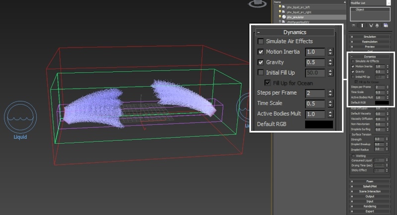
Gravity: 1 and Time Scale: 1
Gravity: 0.5 and Time Scale: 0.5
Set the Default Viscosity to 0.01. Viscosity emulates thickness - the higher this value is, the more the liquid will resemble thick mud, honey or tar.
Phoenix supports the simulation of liquids with varying viscosity. If you'd like to give different viscosity values to the milk and chocolate liquids, you simply need to select the Phoenix Liquid Sources, enable Viscosity and give the parameter a value. Also, don't forget to enable the Grid and Particle Viscosity channel output from the Output rollout . At this point, the Dynamics → Viscosity Diffusion parameter controls how the two thicknesses of the liquids emitted from the two sources will mix.
Set the Surface Tension parameter values as follows:
Strength: 0.5;
Droplet Breakup: 1.0;
Droplet Radius: 2.5.
Strength controls the force produced along the curvature of the liquid surface - this keeps the liquid from breaking into individual particles when a force is applied to it.
Droplet Breakup controls balances between the liquid forming tendrils or droplets. Larger values will produce more droplets.
Droplet Radius controls the radius of the droplets formed by the Droplet Breakup parameter (in voxels). Therefore, if you increase the resolution of the grid, you should also increase the Droplet Radius.
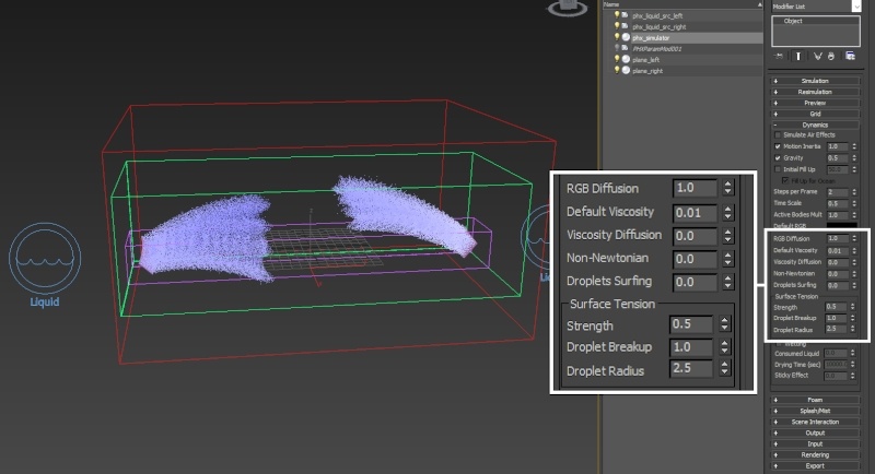
No Viscosity and Surface Tension tweaks
With Viscosity and Surface Tension tweaks
Enable RGB on both Phoenix Sources.
Set the RGB color for the LEFT source to pure white (255, 255, 255).
Set the RGB color for the RIGHT source to black (1, 1, 1). The value is set to (1, 1, 1) instead of (0, 0, 0) so we can preview the channel in the Preview rollout of the simulator.
Make sure that the color is GRAYSCALE - in other words, confirm that the R, G and B values are the same. If you accidentally enter a value such as (255, 255, 240), this will affect the color of the material later on by offsetting the Hue and giving an undesired tint. This could potentially turn into a very insidious, hard to track down problem.
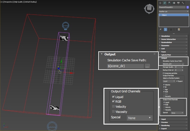
Enable RGB channel export from the Output rollout of the Phoenix Simulator.
If disabled, the RGB channel will not be cached to disk and cannot be queried by the Phoenix Grid Texture later on.
To get a viewport preview of the RGB channel, disable Mesh Preview (if enabled) and enable RGB at the bottom of the Voxel Preview section. You may also disable all other Voxel Preview channels so they don't interfere.
Disable the Auto Range checkbox (this tries to automatically find the min/max range of each channel and adjust the preview range accordingly). Set the RGB max value to 1.0, and the RGB min value to 0.001.
If you now Start the sim, you should get a preview of the RGB channel in the viewport.
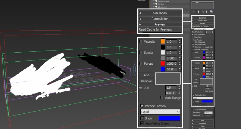
Here is how the RGB channel looks:
At the moment, the emission is too uniform. One way to break the cubic shape up is to use a texture as a modulator for the emission.
Open the Material Editor and create a VRayMtl. Assign it to both poly planes.
Proceed by creating a Stucco texture and piping it into the Diffuse map slot of the VRayMtl.
If you'd like to be able to preview the material in the Viewport, Right-Mouse-Button click the VRayMtl and select the Show Shaded Material option. You may also need to change the Viewport Quality option from Standard to High Quality.
The Stucco settings are described in the steps below.
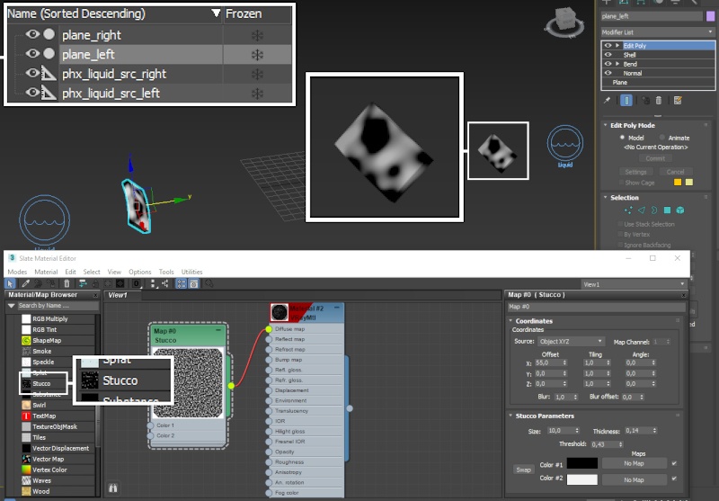
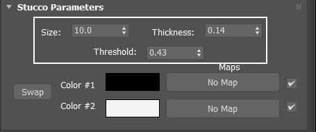
Here are the values for the Stucco Parameters rollout:
Size: 10;
Thickness: 0.14;
Threshold: 0.43.
You may experiment with those - the emission pattern will be heavily affected.
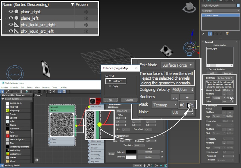
Select one of the Phoenix Sources and Left-Mouse-Button drag from the Stucco output to the Outgoing Velocity Mask parameter.
This will set up the Stucco to work as an emission modulator - black values will emit no liquid, white values will emit with full Outgoing Velocity.
Make sure to choose the Instance setting (as the Copy option will create a copy of this map - you want to use the same texture for both sources instead of being forced to deal with 2 separate Stuccos).
Repeat this step for the other Phoenix Source.
Here's how the emission looks when modulated by the Stucco.
Note that the break-up is static. We will animated the Offset of the Stucco texture to resolve this.
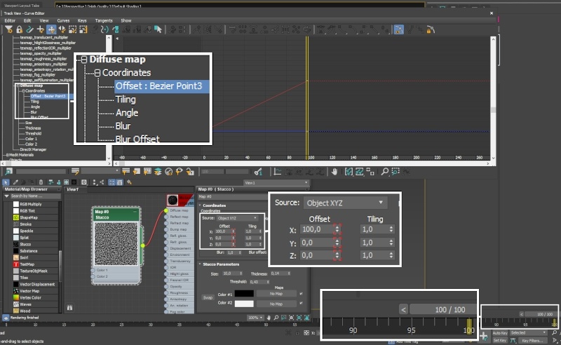
To animate the Offset parameter from the Coordinates rollout of the Stucco texture, simply enable Auto Key from the bottom right of the 3ds Max window, go to frame 100 and set the Offset X value to 100. This should set the Offset X such that it is equal to 0 at frame 0 and 100 at frame 100.
Note that the Offset parameter value does not update on Timeline changes. The best way to make sure that the keyframes are properly set up is to drag the Time slider at the bottom and look for changes in the Viewport. The texture should be 'swimming' over the surface of the source geometry.
Consider setting the tangents for the Offset animation to Linear.
If you can't see the animation curve for the Offset in the Curve Editor, go to View → Filters and disable all options under the Show Only dialog. You should now be able to find it under the VRayMaterial → Diffuse map parameters.
Here's the emission when modulated by the Stucco with an animated Offset parameter.
Mesh Smoothing Options
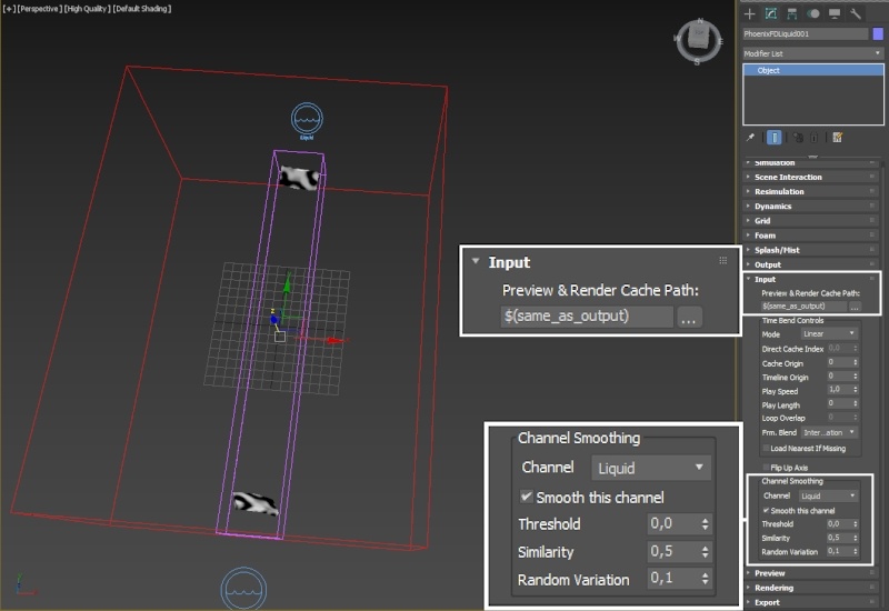
Enable Liquid Channel Smoothing from the Input rollout. This option applies a smoothing algorithm over the cache as its read back into the Simulator for preview and rendering.
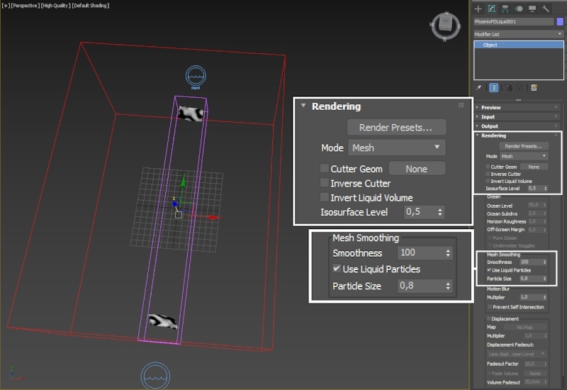
Open the Rendering rollout of the Phoenix Simulator and set the Smoothness parameter to 100. This is yet another smoothing option dedicated especially to meshes, available to you to combat grid artifacts and produce a clean liquid surface.
Enable Use Liquid Particles and set the Particle Size to 0.8. The Liquid Particles option allows the meshing algorithm to produce a surface with varying thickness. You can use the Particle Size parameter to control the thickness of the mesh.
No Smoothing
Smoothness 100 + Use Liquid Particles
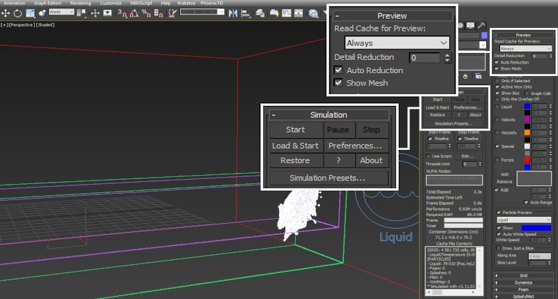
We are now ready to Start the simulation at the final Cell Size of 0.64cm.
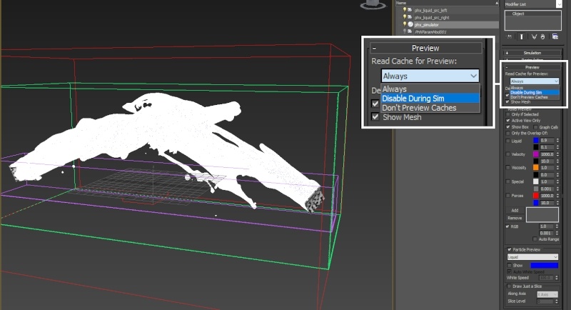
You may want to set the Preview rollout → Read Cache for Preview option to Disable During Sim - this will save some time as the CPU and Graphics card won't be bogged down by the smoothing operations over the cache files read by the Simulator on each frame.
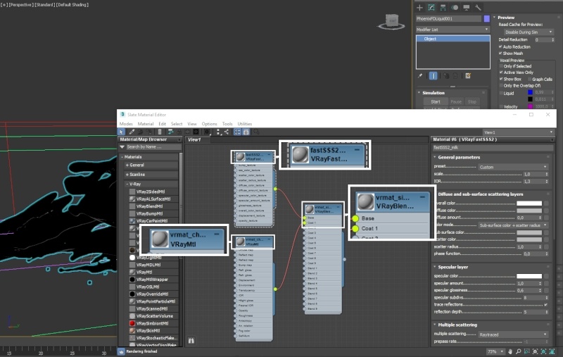
V-Ray Blend Material Setup
Create a VRayBlendMtl and assign it to the Phoenix Simulator.
Then, create two more materials - a VRayFastSSS2 material and a VrayMtl.
Plug the VRayFastSSS2 into the Base slot of the Blend material.
Plug the VRayMtl into the Coat1 slot of the Blend material.
Here's how this setup is going to work: we use a Phoenix Grid Texture to read the RGB channel of the Simulator and use that as the blending factor between the two materials. The VrayFastSSS2 material will be revealed where the RGB channel is black, the VRayMtl will show where the RGB is white, and the RGB values in-between will produce a mix between the two.
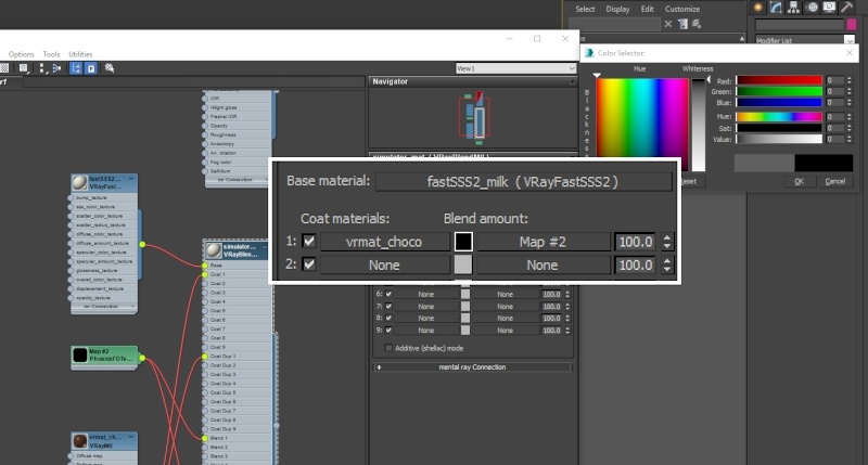
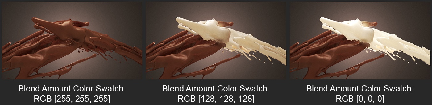
In addition to the Phoenix Grid Texture, the color swatch on the Vray Blend Material will have an effect on the blending factor for the Milk and Chocolate materials. By default it's set to RGB (128, 128, 128) - this will cause the Chocolate material to partially show through the milk regardless of the RGB channel's value.
This will be especially noticeable in case one of the two materials is purely refractive (i.e. water) and the other is opaque. The refractive material will be tinted with the coat.
You may set the value to a dark color if prefer to have this effect disabled.
Please check the image below for comparisons.
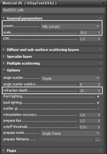
Here are the settings for the VRayFastSSS2 material.
The Preset parameter is set to Milk (whole) and the Scale is increased to 10 to produce a thicker appearance.
The Refraction Depth parameter is also increased to 10.
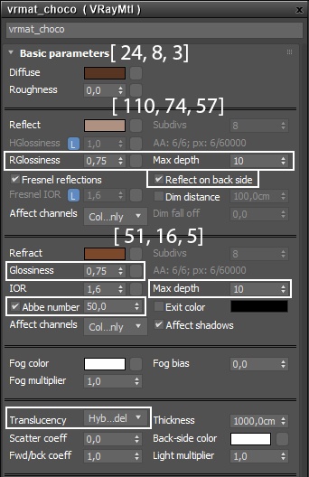
For the VRayMtl used for the chocolate, the following settings are used:
Diffuse: RGB (24, 8, 3);
Reflection color: (110, 74, 57);
Reflection Glossiness: 0.75;
Reflection Max Depth: 10;
Reflect on backside: Enabled;
Refraction Color: (51, 16, 5);
Refraction Glossiness: 0.75;
Refraction Max Depth: 10;
Dispersion Abberation: Enabled, with a value of 50.
Translucency is set to Hybrid Model - this setting is optional and can be omitted for shorter render times.
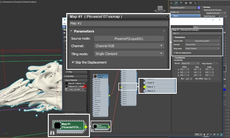
Lastly, create a Phoenix Grid Texture and plug it into the Blend 1 slot of the VRayBlendMtl.
Set the Channel parameter to Channel RGB so the grid texture knows to read the RGB channel of the simulated cache files.
As previously stated, the logic here is fairly simple - the Base (milk) material will appear where the RGB channel is white, and the Coat (chocolate) material will appear where the RGB is black.
Camera
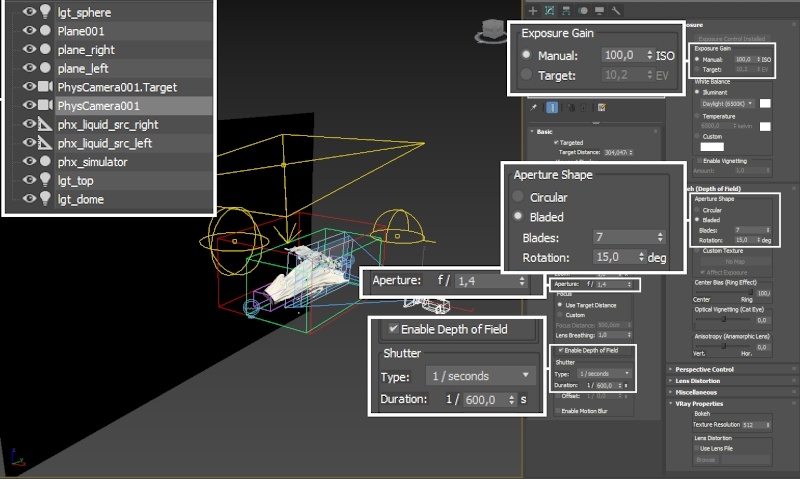
The camera is placed right in front of the Phoenix Simulator. You can experiment with different angles.
Exposure Gain is set to Manual 100 ISO and the Shutter speed to 1/600 - this should give you a balanced exposition that you can easily tweak further in a compositing package or the V-Ray Frame Buffer.
Aperture is reduced to 1.4 and Depth of Field is enabled. A small aperture in conjunction with Depth of Field produces a beautiful blooming effect of the highlights that are out of focus.
To further tweak this, the Aperture Shape is set to Bladed, with the Blades set to 7 and the Rotation to 15 degrees.
Feel free to experiment with these settings and find something that suits your taste.
Lighting
The lighting in the scene is crucial for a good looking render.
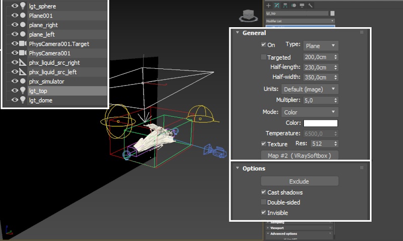
The key light in this scene is the V-Ray Plane light, placed above of the simulation grid.
The Half-Length/Width values are: [230cm, 350cm].
The Intensity Multiplier is set to 5 and the Invisible option is enabled under the Options rollout.
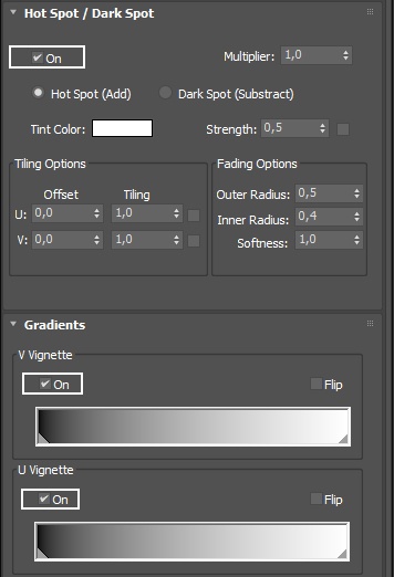
A VRaySoftbox texture is applied to modulate the light intensity. The parameters for it are provided in the next step of this tutorial.
Enable the Hot Spot/Dark Spot option on the VRaySoftbox texture.
Make sure to also enable V/U Vignetting - this will smooth out the light emission at the edges of the VRay Rect Light.
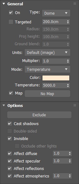
We also have a V-Ray Dome light in the scene.
The Multiplier value is set to 1 and the Mode is set to Temperature: 5000.
The Invisible option is enabled under the Options rollout.
However, you may want to take advantage of a good HDR card to bring your image to life.
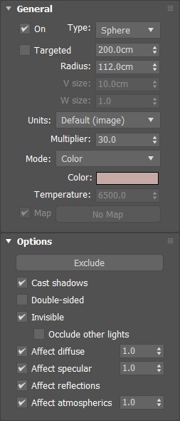
Finally, a VRay Sphere Light is used for backlighting. Recall that the milk is using a VRay FastSSS2 shader - the backlight will bring out the translucency and help produce more believable shading.
The Multiplier value is set to 30 and the Mode is set to Color RGB (144, 105, 98).
The Invisible option is enabled under the Options rollout.
A regular poly plane is used as a backdrop for rendering. A default VRayMtl is assigned to it with the only change being the value of the Diffuse color RGB (10, 10, 10).
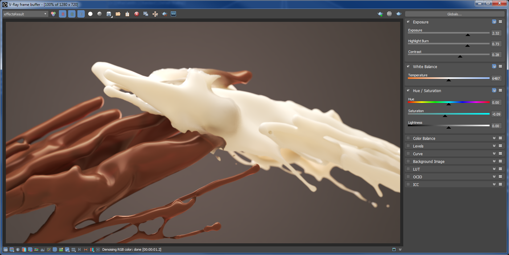
V-Ray Frame Buffer
Now that we are happy with the render result, we can make small adjustments to the image directly from the V-Ray frame buffer.
Here we have tweaked the Exposure, the White Balance and the Hue/Saturation to make the image more interesting.
Also, a V-Ray Denoiser Render Element is added to the final image. The Denoiser takes an existing render and applies a denoising operation to it after the image is completely rendered in order to remove the noise in the image.
Experiment with these parameters to find the best photorealistic look for your beautiful Chocolate Milk fusion.
Final Result
And here is the final result.