This page provides information on the Dynamics rollout for liquids.
Overview
This rollout controls the fluid's motion parameters, which affect the fluid’s behavior when simulating.
UI Path: ||Select Liquid Simulator object|| > Modify panel > Dynamics rollout
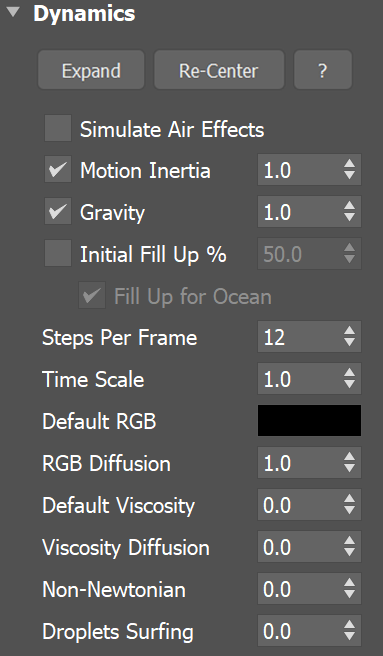
Parameters
Expand – Opens a floating dialog that contains the selected rollout and automatically folds the command panel rollout.
Re-Center – Resets the position of the floating rollout.
? – Opens up the help documents for the Liquid Dynamics.
Simulate Air Effects | simair – When enabled, turns on the built-in air simulator for the areas in the simulation grid which are not full of liquid. The air velocity can be affected by the liquid movement, by Sources, or by fast moving obstacles inside the Simulator. In turn, the air velocity will affect and carry splash, mist, and foam particles. Note, however, that no matter how strong the air velocity is, it will not affect the liquid back. So for example you can use Simulate Air Effects when realistic mist is needed in waterfall setups, or stormy ocean scenes. The air simulation can dramatically increase the quality of splash and mist effects.
The air effects stop affecting particles once they exit the Simulator thus altering the particle speed and direction around the Simulator's walls.
Motion Inertia | ext_wind – When enabled, moving the Simulator's object over a series of frames causes inertial forces in the opposite direction of the movement. This allows you to link the Simulator to a moving object and keep the size of the grid relatively small, as opposed to creating a large grid that covers the entire path of the moving object. Motion Inertia can be used for moving ground and water vehicles, torches, fireballs, rockets, etc. When this option is used together with the Initial Fill Up option and Open Container Wall conditions, a simulation of moving an object over a sea surface can be done. For more information, see the Motion Inertia example below.
When running liquid simulations with the Initial Fill Up option and Open Container Wall conditions, the surface of the generated liquid should remain smooth. If you encounter artifacts in the form of horizontal lines perpendicular to the direction of movement, with Motion Inertia enabled, please ensure that the Scene Scale is reasonable considering the type of effect being simulated. Other possible solutions in case tweaking the scale is not possible are to either increase the Steps Per Frame, or to reduce the Cell Size of the Simulator.
Liquid artifacts usually appear when the liquid particles move a great distance between frames. Increasing the Scene Scale or the Steps Per Frame allows them to stabilize, which in turn keeps the surface smooth.
Gravity | grav, gmul – Phoenix Gravity makes the liquids fall down and makes fire rise up. The Gravity option is a multiplier, so using the default 1.0 will make it behave like real world gravity, setting it to 0.0 will disable its effect completely, and you can also use negative values, which will inverse the gravity effect.
Initial Fill Up | initfill, flevel – When enabled, the container is filled up with liquid when the simulation starts. This option determines the fill-up level, measured in % of the vertical Z size of the Grid. For liquid simulations using Confine Geometry, you can enable Clear Inside on the geometry and liquid will not be created at simulation startup in the voxels inside the geometry.
The liquid created through the Initial Fill Up option will be initialized with the values set for the Default RGB and Default Viscosity parameters below.
Fill Up For Ocean | oceanfill – Changes the Open Container Walls of the Simulator so they would act like there is an infinite liquid volume beyond them. Pressure will be created at the Simulator's walls in order to support the liquid, and if the surface of a wall below the Initial Fill Up level, or the bottom, gets cleared from liquid during simulation, new incoming liquid would be created. You can also animate the Simulator's movement or link it to a moving geometry, and it would act like a moving window over an ocean that stays in place. This way you can simulate moving ships or boats that carry their Liquid Simulator along with them as they sail into an ocean, so you don't need to create one huge long Simulator along their entire path.
In order to eliminate air pockets between Solid geometry and the liquid mesh, this option will automatically set all Solid voxels below the Initial Fill Up level to contain Liquid amount of 1, even if they don't contain any Liquid particles. If you don't want this effect, enable Clear Inside from the Chaos Phoenix Per-Node Properties of the Solid geometry. See the Fill Up For Ocean and Clear Inside example below.
All Simulator walls must be set to Open from the Grid rollout for Fill Up For Ocean to take effect.
Steps Per Frame | spf – Determines how many calculations the simulation will perform between two consecutive frames of the timeline. For more information, see the Steps Per Frame example below.
Steps Per Frame (SPF) is one of the most important parameters of the simulator, with a significant impact on quality and performance. To understand how to use it, keep in mind that the simulation is a sequential process and happens step by step. You cannot take a shortcut to simulate the last frame of a simulation, without first simulating all of the frames that come before it, one by one.
The simulation produces good results if each step introduces small changes to the sim.
For example, if you have an object that is hitting a liquid surface with a high speed, the result will not be very good if at the first step, the object is far away from the water, and at the second step, the object is already deep under the water. You need to introduce intermediate steps, until the object's movement becomes small enough that it happens smoothly across all steps for that frame.
The SPF parameter creates these steps within each frame. A value of 1 means that there are no intermediate steps, and each step is exported into the cache file. A value of 2 means that there is one intermediate step, i.e. each second step is exported to the cache file, while intermediate steps are simply calculated, but not exported.
Increasing the Steps Per Frame (SPF) also comes with significant trade-offs to performance and detail.
A higher SPF decreases performance in a linear way. For example, if you increase the SPF twice, your simulation will take twice as long. However, quality does not have a linear relation to SPF.
For maximum detail, it is best to use the lowest possible SPF that simulates without any of the issues described in the tip box below, since each additional step kills fine details. For more information, please refer to the Phoenix Explained docs.
Signs that the Steps Per Frame (SPF) needs to be increased include:
- Liquid simulations that have too many single liquid particles.
- Liquid simulations that appear torn and chaotic.
- Liquid simulations of streams that have visible steps or other periodical artifacts.
- Fire/Smoke simulations with artifacts that produce a grainy appearance.
More often than not, these issues will be caused by the simulation moving too quickly (e.g. the emission from the source is very strong, or the objects in the scene are moving very fast). In such cases, you should use a higher SPF.
Time Scale | timescale – Specifies a time multiplier that can be used for slow motion effects. For more information, see the Time Scale example below.
In order to achieve the same simulation look when changing the Time Scale, the Steps Per Frame value must be changed accordingly. For example, when decreasing the Time Scale from 1.0 to 0.5, Steps Per Frame must be decreased from 4 to 2. All animated objects in the scene (moving objects and sources) must be adjusted as well.
Time Scale different than 1 will affect the Buildup Time of Particle/Voxel Tuners and the Phoenix Mapper. In order to get predictable results you will have to adjust the buildup time using this formula:
Time Scale * Time in frames / Frames per second
Default RGB | lq_default_rgb - The Simulator is filled with this RGB color at simulation start. The Default RGB is also used to color the fluid generated by Initial Fill Up, or by Initial Liquid Fill from the Chaos Phoenix Per-Node Properties of a geometry - both of these options create liquid only at the start of the simulation. During simulation, more colors can be mixed into the sim by using a Phoenix Liquid Source with RGB enabled, or the color of existing fluid can be changed over time by using a Phoenix Mapper. If a Phoenix Liquid Source does not have RGB enabled, it also emits using the Default RGB value.
The RGB Grid Channel or RGB Particle Channel has to be enabled in the Output Rollout for this parameter to take effect.
RGB Diffusion | rgbdiff – Control how quickly the colors of particles are mixed over time during the simulation. When it's set to 0, each FLIP liquid particle carries its own color, and the color of each individual particle does not change when liquids are mixed. This means that if red and green liquids are mixed, a dotted red-green liquid will be produced instead of a yellow liquid. This parameter allows the colors of particles to change when the particles are in contact, thus achieving uniform color in the resulting mixed liquid. For more information, see the RGB Diffusion example below.
Default Viscosity | lqvisc – Determines the default viscosity of the liquid. Viscosity means how thick the liquid is. Liquids such as honey, syrup, or even thick mud and lava need to be simulated with high viscosity. On the other hand, liquid such as water, beer, coffee or milk are very thin and show have zero or very low viscosity. The Default Viscosity value is used when no viscosity information for the emitted liquid is provided to the Simulator by the Source. Also note that the effect of the viscosity works more strongly with more Steps Per Frame, and also when the grid resolution is lower. Increasing the grid resolution or reducing the Steps Per Frame can make viscous liquid thinner. For more information, see the Viscosity example below.
- All FLIP liquid particles are set to this viscosity value at simulation start. You should use higher viscosity for thicker liquids such as chocolate, cream, etc.
- The Default Viscosity is also used for the fluid generated by Initial Fill Up, or by Initial Liquid Fill from the Phoenix Per-Node Properties of a geometry - both of these options create liquid only at the start of the simulation.
- If a Phoenix Liquid Source does not have Viscosity enabled, it emits using the Default Viscosity value.
- During simulation, liquids of variable viscosity can be mixed into the sim by using a Phoenix Liquid Source with Viscosity enabled.
- The Viscosity Grid Channel export has to be enabled in the Output Rollout for variable viscosity simulations to work.
- The viscosity of existing liquid can be changed over time by using a Phoenix Mapper in order to achieve melting or solidifying of fluids.
- You can shade the liquid mesh or particles using the fluid's viscosity with the help of the Phoenix Grid Texture or Particle Texture.
- It's important to note that using viscosity does not automatically make the liquid sticky. For example, molten glass is viscous, but not sticky at all. Stickiness can be enabled explicitly from the Wetting parameters section. If Stickiness is not enabled, even the most viscous fluid would slide from the surfaces of geometries or from the jammed walls of the Simulator.
Viscosity Diffusion | viscdiff - Phoenix supports sourcing of fluids with different viscosity (thickness) values. This parameter specifies how quickly they blend together. A low value will preserve the distinct viscosities, while a high value will allow them to mix together and produce a fluid with a uniform thickness.
Non-Newtonian | nonnewt – Modifies the viscosity with respect to the liquid's velocity to overcome the conflict between viscosity and wetting, where a high viscosity of real liquids prevents wetting. Non-Newtonian liquids are liquids that behave differently at different velocities. This parameter accounts for this behavior by decreasing the viscosity in areas where the liquid is moving slowly and retains a higher viscosity where the liquid is moving quickly. For example, to cover a cookie with liquid chocolate, high viscosity is needed in the pouring portion of the motion to obtain the curly shape of the chocolate as it lands on the cookie and begins to settle down. On the other hand, a smooth chocolate is needed to settle in over the cookie without roughness and holes. If the viscosity is high enough, the chocolate might look right during the pouring and settling motions but won't settle in to form a smooth thin layer over the cookie. This parameter decreases the viscosity where the liquid is moving slowly (over the surface of the cookie) while keeping the faster-moving stream tight and highly viscous. For more information, see the Non-Newtonian example below.
Droplets Surfing | dsurf – This parameter affects the liquid and the splash particles, controlling how long a particle hovers on the surface before it merges with the liquid. The parameter is used mostly in ocean/wave simulations. For more information, see the Droplets Surfing example below.
Example: Motion Inertia
The following video provides examples of moving containers with Motion Inertia enabled to show the differences between values of 0, 0.5, and 1.0.
Software used: Phoenix 4.30.00 Official Release
Example: Fill Up For Ocean and Clear Inside
This example shows the Liquid voxels, with a submerged Solid ellipsoid. There are never FLIP particles inside it, but disabling Clear Inside will fill it with Liquid voxels so the liquid mesh can intersect it.
![]()
![]()
Example: Steps Per Frame
The following video provides examples to show the differences of Steps Per Frame values at 1, 5, and 15.
Software used: Phoenix 4.30.01 Nightly (02 Oct 2020)
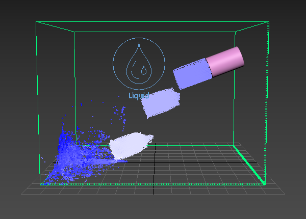
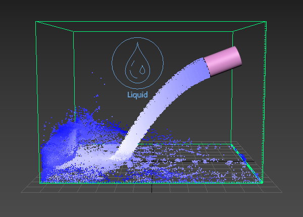
Here is the difference between Steps Per Frame values of 1 and 10 when a Source emits liquid with high velocity.
Example: Time Scale
The following video provides examples to show the differences of Time Scale with values of 0.3, 1.0, and 2.0.
Software used: Phoenix 4.30.01 Nightly (02 Oct 2020)
Example: RGB Diffusion
The following video provides examples to show the differences of RGB Diffusion with values of 0.0, 0.5, and 1.0.
Software used: Phoenix 4.30.01 Nightly (02 Oct 2020)
Example: Default Viscosity
The following video provides examples to show the differences of Default Viscosity with values of 0.0, 0.5, and 1.0.
Software used: Phoenix 4.30.01 Nightly (02 Oct 2020)
Example: Non-Newtonian
The following video provides examples to show the differences of Non-Newtonian with values of 0, 0.1, and 1.0.
Software used: Phoenix 4.30.01 Nightly (02 Oct 2020)
Example: Droplets Surfing
The following video provides examples to show the differences of Droplets Surfing with values of 0.0, 0.5, and 1.0.
Software used: Phoenix 4.30.00 Official Release
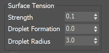
Surface Tension
Strength | lqsurft – Controls the force produced by the curvature of the liquid surface. This parameter plays an important role in small-scale liquid simulations because an accurate simulation of surface tension indicates the small scale to the audience. Lower Strength values will cause the liquid to easily break apart into individual liquid particles, while higher values will make it harder for the liquid surface to split and will hold the liquid particles together. With high Strength, when an external force affects the liquid, it would either stretch out into tendrils, or split into large droplets. Which of these two effects will occur is controlled by the Droplet Formation parameter. For more information, see the Surface Tension example below.
Droplet Formation | lqstdropbreak – Balances between the liquid forming tendrils or droplets. When set to a value of 0, the liquid forms long tendrils. When set to a value of 1, the liquid breaks up into separate droplets, the size of which can be controlled by the Droplet Radius parameter. For more information, see the Droplet Formation example below.
Droplet Radius | lqstdroprad – Controls the radius of the droplets formed by the Droplet Formation parameter, in voxels. This means that increasing the resolution of the Simulator will reduce the overall size of the droplets in your simulation.
Increasing the Droplet Radius can dramatically slow down the simulation. Please use it with caution.
Example: Surface Tension
The following video provides examples to show the differences of Surface Tension with values of 0.0, 0.07, 0.28 and Droplet Formation with value of 0.0.
Software used: Phoenix 4.30.01 Nightly (02 Oct 2020)
Example: Droplet Formation
The following video provides examples to show the differences of Droplet Formation with values of 0.0, 0.5, 1.0 and Surface Tension with value of 0.1.
Software used: Phoenix 4.30.01 Nightly (02 Oct 2020)
Wetting
The simulation of wetting can be used in rendering for blending wet and dry materials, depending on which parts of a geometry have been in contact with the simulated liquid. Wetting can also change the behavior of a simulated viscous liquid and make it stick to geometries.
The wetting simulation produces a particle system called WetMap. Wetmap particles are created at the point of contact between the liquid and the scene geometry, and can be rendered using a Particle Texture map.
When used with a Blend Material, the Particle Texture acts as a mask to blend between two materials, for example, a wet material and a dry surface material. This way, geometry covered by WetMap particles can appear wet, and the rest of the geometry can appear dry.
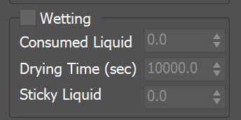
Wetting | wetting – Enables the wetting simulation. The liquid will leave a trail over the surfaces of bodies it interacts with.
Consumed Liquid | lq2wet – Controls how many liquid particles disappear when creating a single WetMap particle. The main purpose of this parameter is to prevent long visible tracks from being left by a single liquid particle. For more information, see the Consumed Liquid example below.
Drying Time (sec) | drying – Controls the drying speed in seconds. The WetMap particles are born with a size of 1, and if they are in an air environment, the size decreases until it reaches zero after the time specified with this parameter.
Sticky Liquid | wetdyn – This option produces a connecting force between the WetMap particles at the geometry surface and nearby liquid particles. For more information, see the Sticky Liquid example below.
Geometry transforming or deforming at a high velocity may cause some or all of the Wetting particles stuck to it to disappear. To resolve this, dial up the Steps Per Frame parameter from the Dynamics tab of the Simulator.
Example: Consumed Liquid
The following video provides examples to show the differences of Consumed Liquid values of 0, 0.1, and 0.3.
Software used: Phoenix 4.30.01 Nightly (02 Oct 2020)
Example: Sticky Liquid without Viscosity
The following video provides examples to show the differences of Sticky Liquid values of 0, 0.5, and 1, when the Viscosity is set to 0.
Software used: Phoenix 4.41.02 Nightly (24 Jun 2021)
Example: Sticky Liquid and Viscosity
The following video provides examples to show the differences of Viscosity values of 0.1, 0.5, and 1.0 and Sticky Liquid with value of 1.0.
Software used: Phoenix 4.41.02 Nightly (24 Jun 2021)
Example: Sticky Liquid with different amount of fluid
The following video provides examples to show the differences of Surface Force values of 50, 500, and 1000, Sticky Liquid with value of 0.5 and Viscosity with value of 0.3.
Software used: Phoenix 4.30.01 Nightly (02 Oct 2020)
Active Bodies
Note that interaction between Active Bodies and the Phoenix Fire/Smoke Simulator is not supported.
Chaos Phoenix can make a ship, or ice cubes, or other geometry float in water using the Active Bodies feature, which introduces Rigid Body Dynamics for specified Active Body objects. Phoenix can even simulate waves that can carry Active Body objects around, or wash them away.
To use Active Bodies, you’ll need to create an Active Body Solver component, and specify the scene geometry which will partake in the Active Bodies simulation. Then, in the simulator’s Dynamics rollout, enable the Active Bodies parameter, and specify the Active Body Solver node.
You can then set the density and other Active Body properties in the Phoenix Per-Node Properties menu for each Active Body object.
The Active Bodies simulation currently supports interaction between scene geometry and the Phoenix Liquid Simulator. When an object is selected as an Active Body, the simulation both influences and is influenced by the Active Body's movement.
For more information on Active Bodies, please check out the Active Body Solver and the Active Bodies Setup Guide.
Active Bodies | use_activeBodySolverNode – Enables the simulation of Active Bodies.
Active Body Solver | activeBodySolverNode – Specifies the Active Body Solver node holding the objects to be affected by the Phoenix Simulation.

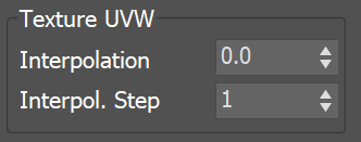
Texture UVW
The main purpose of the Texture UVW feature is to provide dynamic UVW coordinates for texture mapping that follow the simulation. If such simulated texture coordinates are not present for mapping, textures assigned to your simulation will appear static, with the simulated content moving through the image. This undesired behavior is often referred to as 'texture swimming'.
UVW coordinates are generated by simulating an additional Texture UVW Grid Channel which has to be enabled under the Output rollout for the settings below to have any effect.
The custom UVW texture coordinates can be used for advanced render-time effects, such as recoloring of mixing fluids, modifying the opacity or fire intensity with a naturally moving texture, or natural movement of displacement over fire/smoke and liquid surfaces. For more information, please check the Texture mapping, moving textures with fire/smoke/liquid, and TexUVW page.
Interpolation | texuvw_interpol_influence – Blends between the UVW coordinates of the liquid particle at time of birth and its UVW coordinates at the current position in the Simulator. When set to 0, no interpolation will be performed - as a consequence, textures assigned to the fluid mesh will be stretched as the simulation progresses. This is best used for simulations of melting objects. When set to 1, the UVW coordinates of the fluid mesh will be updated with a frequency based on the Interpol.Step parameter - this will essentially re-project the UVWs to avoid stretching but cause the textures assigned to the fluid to 'pop' as the re-projection is applied. If you intend to apply e.g. a displacement map to a flowing river, set this parameter to a value between 0.1 and 0.3 - this will suppress both the effects of stretching and popping. See the Interpolation example below.
Interpol. Step | texuvw_interpol_step – Specifies the update frequency for the UVW coordinates. When set to 1, the UVWs are updated on every frame, taking into account the Interpolation parameter. See the Interpolation Step example below.
Example: Interpolation
The following video provides examples to show the differences of Interpolation values of 0, 0.1, and 1, and an Interpolation Step with value of 1.0.
Software used: Phoenix 4.30.01 Nightly (02 Oct 2020)
Example: Interpolation Step
The following video provides examples to show the differences of Interpolation Step values of 1, 3, and 6, and an Interpolation with value of 1.0.
Software used: Phoenix 4.30.01 Nightly (02 Oct 2020)