Dynamics

This page provides information on the Dynamics rollout.

Overview

---

This rollout controls the dynamics parameters for simulations, which affect the fluid’s behavior when simulating. The Dynamics rollout can be accessed in the Attribute Editor when a PhoenixFDSim object is selected. For liquid-specific dynamics, see the Liquid Dynamics rollout.

Parameters

---

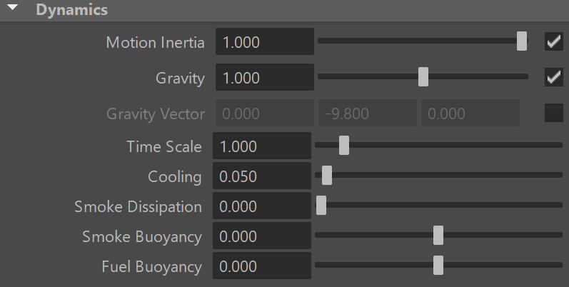
Motion Inertia | windFromMovement – When enabled, moving the simulator object over a series of frames causes inertial forces in the opposite direction of the movement. This allows you to link the simulator to a moving object and keep the size of the grid relatively small, as opposed to creating a large grid that covers the entire path of the moving object. Motion Inertia can be used for moving ground and water vehicles, torches, fireballs, rockets, etc. When this option is used together with the Initial Fill Up option and Open Container Wall conditions, a simulation of moving an object over a sea surface can be performed. For more information, see the Moving Geometry vs. Moving Simulator section of the Tips and Tricks page.

Gravity | gravity, gravityEnbl – Phoenix Gravity makes the liquids fall down and makes fire rise up. In fire/smoke simulations it creates velocities depending on the Temperature channel. In voxels where the Temperature is above 300 (in Kelvins, which is room temperature), Gravity will create upwards velocities. Where Temperature is below 300, the opposite will happen - velocities will be created pointing downwards. The hotter the fluid, the faster it will rise, and the cooler the fluid below 300, the faster it will fall down. The Gravity option is a multiplier, so using the default 1.0 will make it behave like real world gravity, setting it to 0.0 will disable its effect completely, and you can also use negative values, which will inverse the gravity effect.

Gravity Vector | gravityVec, gravityVecEnbl – When enabled, a custom gravity force vector is used instead of the default one (0, -9.8, 0).

Time Scale | timeScale – Specifies a time multiplier that can be used for slow motion effects.

Cooling | cooling – This parameter controls the cooling of the fluid due to radiation. The temperature in the simulator is gradually reduced until it reaches 300.

Smoke Dissipation | smokeDissipation – Used in simulations where the smoke needs to disappear, e.g. steam, clouds, etc. If you set this parameter to the maximum value of 1, the smoke will disappear immediately.

Smoke Buoyancy | smokeBuoyancy – The buoyancy of the smoke. Positive values make the smoke move upwards. Negative values make it move downwards.

Fuel Buoyancy | fuelBuoyancy – Specifies the buoyancy of the fuel.

Vorticity

---

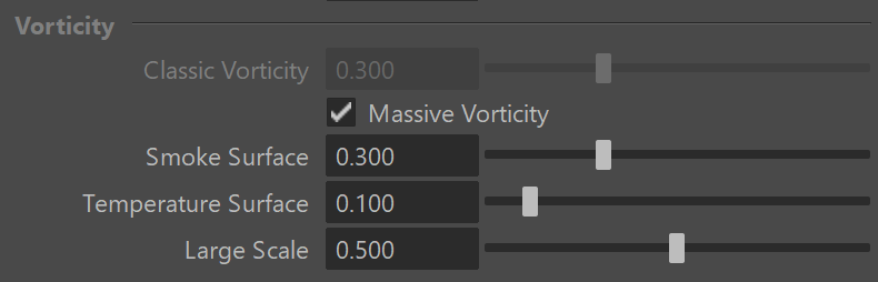
Classic Vorticity | vorticity – Adds small-scale detail that is dissipated naturally by the grid-based simulation. Prevents the simulation from becoming smooth and laminar. Unlike Turbulence, which does not care about the fluid's motion at all, the Classic Vorticity algorithms works depending on the velocity of the simulation and changes the velocity field in order to reinforce vortices and add more detail to the simulation. For more information, see the Vorticity example below.

Massive Vorticity | vorticityModV  – This mode generally improves the vorticity detail and behavior. Unlike Classic Vorticity which reinforces vortices throughout the grid, the Massive Vorticity gets applied more strongly only to some parts of the fluid, making a difference between thin air with no smoke or temperature, the smoke and temperature's surface, and the inside volume of fluids. The added detail is equally strong for both the fast and the slow moving parts of the fluid. Massive Vorticity also does not produce a boiling effect that is present in the Classic Vorticity algorithm, which tears up the slower moving parts of the fluid excessively and stops the fluid's motion. For more information, see the Vorticity example below.

Smoke Surface/Temperature Surface | vorticitySurfSm / vorticitySurfT – These options create vortices only on the smoke/temperature channel's surface without disturbing the flow in the inner volume of the fluid. This way massive vorticity won't block the fluid's general motion and break the fluid apart as the classic vorticity does. It's split into separate smoke and temperature multipliers for additional flexibility. For example, in a fire-only simulation, you need to use Temp. Surface, while in a smoke-only simulation, you need Smoke Surface instead.

Large Scale | vorticity_low – The large-scale multiplier reinforces the big vortex flows in the inner part of the fluid. The effect is similar to what higher Conservation quality can achieve, with the difference that the Large Scale vorticity does not respect obstacles, so it might not be suitable in a more complicated setup. For more information, see the Vorticity example below.

Randomize

---

These options add random fluctuations in the fluid's velocity for each grid voxel.

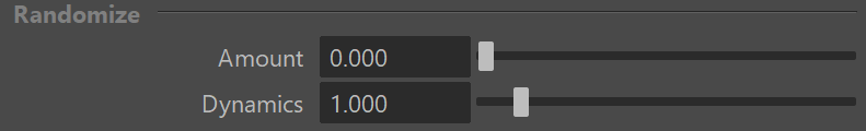
Amount | randAmount – The amount of randomization. Only the velocity length is changed; the velocity direction remains the same.

Dynamics | randDynamics – The speed of change of the fluctuations. The higher the value, the faster the random noise will change over time.

Fluidity (Conservation)

---

The conservation process gives the fluid its characteristic swirling motion. It transforms straight-line movement of the fluid into swirling vortices. The higher the strength of the conservation, the farther the motion forces will be propagated throughout the container, so a movement in one point will cause the fluid to start moving at a distance too. The conservation directs smoke and fire into realistic shapes and helps liquids to support their own weight when at rest, and to fill up a volume they are poured into.

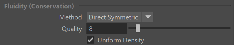
Method | conservMethod – Specifies the method for simulating the conservation. For more information, see the Conservation Method Types example below.

Direct Symmetric – This method has a long range and can transfer movement and pressure from one point of the grid can to distant parts of the grid. It also achieves strong conservation without having to boost the quality too much, and thus the fluid can roll and swirl quite well. Thus it is well suited for simulation of explosions with shockwaves.
Direct Smooth – The smooth method is quite similar to Direct Symmetric. It produces a smoother velocity field and is stronger than Direct Symmetric, but doesn't keep the symmetry that well and it will produce less detail.
Buffered – This method has the weakest conservation strength and shortest range, but produces detail that works well when simulating fire.
PCG Symmetric – This method provides a very strong conservation, but works at a shorter range than the Direct Symmetric method. It actually produces better symmetry than Direct Symmetric and so it can be used to simulate nuclear mushrooms or other effects where high symmetry is crucial. It is also the best method to use for smoke or explosions in general. The Uniform Density option is ignored in this mode, so simulating only fire with this mode may not produce as good results as using the other methods that allow Uniform Density to be enabled.

Quality | conservQuality – Increases the strength of the conservation. It will help cases when the liquid or smoke is losing volume, or the swirling of the smoke needs to be increased. Beware that increasing the quality will slow down the simulation.
For more information, see the Quality example below.

Uniform Density | conservUniform – When enabled, the mass of the fluid will not be considered. Fire simulations work better with this option on, which ignores the mass. However, unchecking this option might be useful for pure smoke simulations or explosions (for fire/smoke simulations the inverse of the temperature is considered the mass; the hotter fluid will be lighter and the cooler fluid will be heavier, just as in nature).

Transport (Advection)

---

Advection is the process that moves the fluid along its velocity inside the grid. A problem of all grid-based simulators is that moving the content of one cell to a new place in the grid will blur the result when the destination lies between cells (and it usually does), thus losing the fine details with each new frame. Phoenix has a number of advection methods that battle this problem in different ways, each with its own pros and cons depending on the situation.

Method | advMethod – Specifies the algorithm used for calculating the advection. For more information, see the Advection Method Types example below.

Forward Transfer – Forward Transfer can help if you are losing fluid volume, but is less detailed. Multi-Pass produces the best fluid details and keeps the smoke sharp, making it best for large scale explosions and simulations when sharpness is important.
Multi-Pass – This less dissipative method produces more fine details and keeps the smoke interface sharper compared to other methods. This method is recommended for large scale explosions, veil-like smoke, pyroclastic flows, and all other situations where sharpness is important.

Steps Per Frame (SPF) | advSPF – Determines how many calculations the simulation will perform between two consecutive frames of the timeline. For more information, see the Steps per Frame examples below.